GENESIS Tutorial 4.1 (2022)
Analysis of DCD file by the user’s Fortran programming
Preparation
After running MD simulations, the resulting trajectory data are saved in DCD files. GENESIS provides several built-in analysis tools, mainly for calculating commonly used quantities such as distances, angles, RMSD, and so on. However, if you need to analyze less typical (“minor”) quantities that are not supported by the default tools, you will need to write your own scripts or programs. In this tutorial, we will learn how to analyze DCD trajectory data by modifying a simple sample Fortran program.
All the files required for this tutorial are hosted in the GENESIS tutorials repository on GitHub. If you haven’t downloaded the files yet, open your terminal and run the following command (see more in Tutorial 1.1):
$ cd ~/GENESIS_Tutorials-2022
# if not yet
$ git clone https://github.com/genesis-release-r-ccs/genesis_tutorial_materials
If you already have the tutorial materials, let’s go to our working directory:
$ cd genesis_tutorial_materials/tutorial-4.1
$ ls
ionized.pdb  run.dcd  sample.f90
1. What is contained in the DCD file?
In this directory, you will find both PDB and DCD files. The system is very
small — just one protein (chignolin), water molecules, and ions — totaling 2,382
atoms. The trajectory contains 50 frames, generated by GENESIS and processed
using the crd_convert tool, with water and ions wrapped into the unit cell.
# Take a look at the trajectory using VMD
$ vmd ionized.pdb -dcd run.dcd
Let’s take a quick look at the DCD file using the less command:
# Take a look at the contents in the DCD file
$ less run.dcd
You’ll notice that DCD files are unreadable — they are in binary format, not human-readable text. This is intentional: molecular dynamics (MD) simulations produce large amounts of trajectory data, and storing them in binary keeps the file size much smaller than text (ASCII) format.
Despite being unreadable, the binary DCD format follows a standardized structure. That means we can still extract useful information from it — such as the number of atoms, number of frames, and coordinates in each frame.
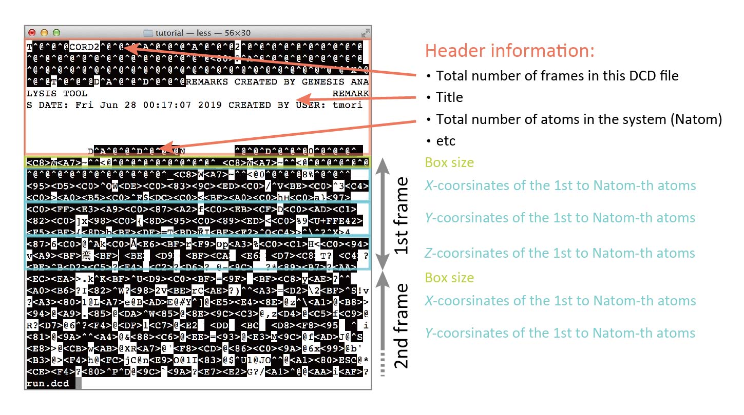
The DCD file begins with a header section that includes general information, such as the total number of frames and the number of atoms in the system. This is followed by the coordinate data for each frame: box dimensions (if available), and then the x-, y-, and z-coordinates of all atoms for that frame. This structure is repeated for every frame in the trajectory.
It’s important to note that DCD files do not contain additional metadata such as atomic masses, residue names, or atom names — that information must be retrieved from a corresponding PDB or PSF file.
2. An example program
2. Example Program
In this directory, you will find an example (sample.f90) written in the
Fortran programming language 1, 2. If you are not very familiar
with coding, don’t worry — try to follow the logic line by line.
This program opens a DCD file (run.dcd) and reads the box dimensions and the
atomic coordinates for each frame. It doesn’t perform any analysis yet. Instead,
you will see a comment line in the code: ! Analyze the snapshot here.
This is where you can insert your own calculations to analyze physical
quantities of interest.
In the next section, we’ll walk you through a concrete example of how to modify this program to calculate the distance between two atoms.
# View the sample program
$ less sample.f90

! DCD analysis program
!
program main

  implicit none
  integer              :: i, natom
  integer(4)           :: dcdinfo(20), ntitle
  real(4), allocatable :: coord(:,:)
  real(8)              :: boxsize(1:6)
  character(len=4)     :: header
  character(len=80)    :: title(10)

  open(10, file='run.dcd', form='unformatted', status='old')
  read(10) header, dcdinfo(1:20)
  read(10) ntitle, (title(i),i=1,ntitle)
  read(10) natom

  allocate(coord(1:3,1:natom))

  do i = 1, dcdinfo(1)
    read(10) boxsize(1:6)
    read(10) coord(1,1:natom)
    read(10) coord(2,1:natom)
    read(10) coord(3,1:natom)

    ! Analyze the snapshot here

  end do
  close(10)

end program main
In this example, the box size for each frame is read using the line:
read(10) boxsize(1:6). However, if your simulation was run with the setting
boundary = NOBC (i.e., no boundary conditions), then the box size information
will not be included in the DCD file. In that case, you should comment out or
remove this line to avoid a read error.
Also note that this program is designed to read DCD files written in
little-endian format. Most modern computers, such as those with Intel CPUs,
use little-endian encoding. However, some machines — such as Fujitsu
systems — produce big-endian binary files. If you’re working on such a
system, you must modify the open statement to include the following option:
convert='big_endian'. This ensures the DCD file is read correctly regardless
of the system architecture.
3. Distance analysis
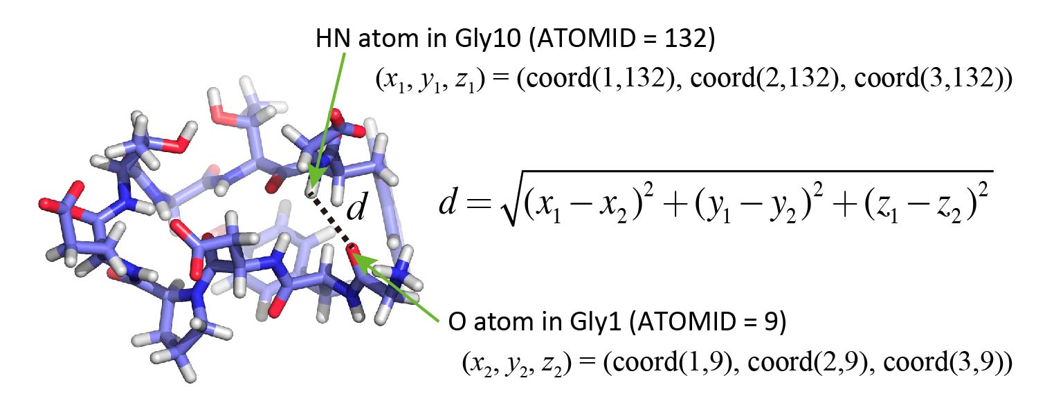
Now, let’s analyze the distance between two specific atoms: the HN atom of Gly10
and the O atom of Gly1, whose ATOMIDs are 132 and 9, respectively (as seen in
the PDB file).
In the Fortran program, the coordinates of atoms in each snapshot are
stored in a two-dimensional array named coord. In this array:
coord(1, i)holds the x-coordinate of the i-th atom,coord(2, i)holds the y-coordinate,- and
coord(3, i)holds the z-coordinate.
To calculate the distance between two atoms, you can use the standard formula
based on the square root (sqrt) of the sum of squared differences.
Let’s now edit the program. You can use any text editor you like, such as vi, emacs, or gedit.
Add the parts as shown below. But don’t just copy and paste the code! Instead, try to understand the meaning of each line and type it in yourself. This will help you better understand how the program works and how to modify it for other types of analyses.
! ...

  integer              :: i, natom, atm1, atm2
  integer(4)           :: dcdinfo(20), ntitle
  real(4), allocatable :: coord(:,:)
  real(8)              :: boxsize(1:6), dist, dx, dy, dz

! ...

  allocate(coord(1:3,1:natom))

  atm1 = 132
  atm2 = 9
  do i = 1, dcdinfo(1)
    read(10) boxsize(1:6)

! ...

    ! Analyze the snapshot here
    dx   = coord(1,atm1) - coord(1,atm2)
    dy   = coord(2,atm1) - coord(2,atm2)
    dz   = coord(3,atm1) - coord(3,atm2)
    dist = dsqrt(dx*dx + dy*dy + dz*dz)

    write(20,*) i, dist
  end do
  close(10)
! ...
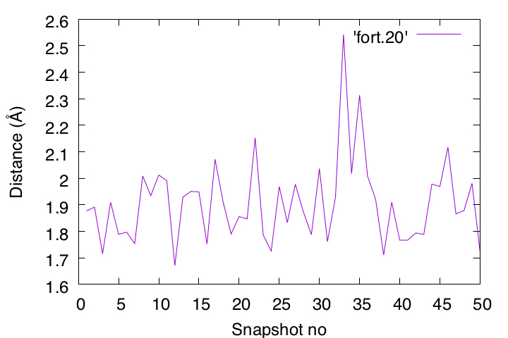
Now, go ahead and compile the source code, and then run the program. Because we
used write(20,*) in the code, the output will be saved to a text file called
fort.20. You can take a look at it with the less command, or even plot the
values using Gnuplot.
Also, don’t forget to open the peptide structure in VMD and double-check whether the data you plotted matches what you see in the simulation.
# Compile the fortran program
$ gfortran sample.f90
$ ls
a.out  ionized.pdb  run.dcd  sample.f90

# Execute the program
$ ./a.out
$ ls
a.out  fort.20  ionized.pdb  run.dcd  sample.f90
If there is a discrepancy between the data plotted in Gnuplot and the structure displayed in VMD, it may indicate a bug in your program. To catch such bugs, your chemical intuition is also important.
In this example, we are analyzing a pair of atoms that are expected to form a hydrogen bond, so the distance between them should generally be less than 2.5 Å. If you find a frame where the calculated distance exceeds 2.5 Å, take a closer look at that snapshot in VMD. If it still shows hydrogen-bond formation visually, then you should suspect something might be wrong with your program.
Doing these kinds of double- and even triple-checks is crucial to ensure the accuracy of your analysis.
Written by Takaharu Mori@RIKEN Theoretical molecular science
laboratory
Feb. 24, 2022
Updated by Cheng Tan@RIKEN Center for Computational Science
Jun. 19, 2025
References
-
Fortran by Wikibooks (English) ↩
-
Fortran 入門 (Japanese) ↩