GENESIS Tutorial 15.6 (2022)
The enzyme reaction 2: Free-energy calculation
1. Introduction
In this section, we demonstrate the replica-exchange umbrella sampling (REUS) simulation based on a QM/MM potential and calculate the free-energy profile of an enzyme reaction. REUS 1 is one of the enhanced sampling methods, in which multiple MD simulations (replicas) are carried out with different restraint potentials, exchanging them stochastically. In tutorial 12.2, REUS has been performed with classical MM-MD. This tutorial is similar to it but differs in:
- The reaction coordinate is set to a pre-determined minimum energy path (MEP).
- QM/MM-MD simulations are carried out using QSimulate-QM.
Following tutorial 15.5, the method is applied to a proton transfer reaction of dihyroxyacetone phosphate (DHAP) catalyzed by triosephosphate isomerase (TIM) 2. Although the MEP and restart files are provided in the tutorial file, it is recommended to first work on tutorial 15.5, where the MEP is obtained by the string method.
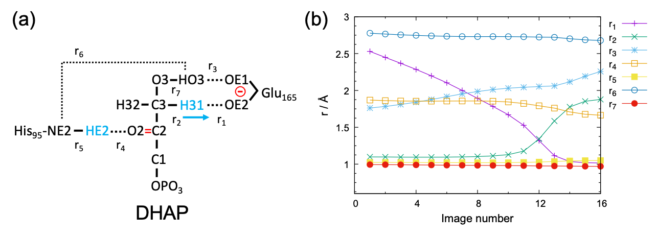
The target proton transfer reaction and selected atomic distances (r1 – r7) are schematically shown in Fig. 1 (a). The variation of r1 – r7 along the MEP is shown in Fig. 1 (b). The figure indicates that r1 – r4 strongly vary along the path, whereas r5 and r7 are rather insensitive. r6 is relatively flat compared to r1 – r4, yet it does change 0.1 Å before and after the reaction. Therefore, the five atomic distances, r1 – r4 and r6 , well represent the reaction coordinate. Here, we carry out the off-lattice REUS using these atomic distances as a collective variable (CV).
2. Setup of window
Download the tutorial file (GENESIS tutorials repository on GitHub), and proceed to tutorial-15.6/1.tim. The directory contains three sub-directories.
$ unzip tutorial22-15.6.zip
$ cd tutorial-15.6/1.tim
$ ls
2.equil/ 4.mep/  5.reus/
2.equil contains psf and pdb files, and a restart file,
$ ls 2.equil
step4.11_qmmm_nvt.rst   step4_nvt_100.pdb   step4_nvt_100.psf
and 4.mep contains the information of the MEP,
$ ls 4.mep/2.analysis
rpath_93.dat
You are welcome to overwrite these files with your results in tutorial
15.5 (or add 5.reus to your tutorial15.5/1.tim). Proceed to
5.reus, and you will find seven sub-directories.
$ cd 5.reus
$ ls
0.window/   2.equil2/          3.prod3/           4.pmf/
1.equil1/   2.equil2_analysis/ 3.prod3_analysis/
Now, let us generate the windows of US,
$ cd 0.window
$ ls
make_window.f90  make_window.sh  win_rr.gpi
make_window.f90 is a fortran program to generate the windows, and
make_window.sh is a script to run the program.
$ cat make_window.sh
#!/bin/bash

gfortran make_window.f90 -o make_window
./make_window -dat ../../4.mep/2.analysis/rpath_93.dat \
              -ds 0.1 -ndim 5 -idx 1,2,3,4,6 > win_rr.log
The first line compiles the program. “gfortran” can be replaced with other fortran compilers. The second line executes the program. The options are:
- -dat : the information of the MEP
- -ds : the interval of window (in Å)
- -ndim : the number of dimensions
- -idx : optionally specifies which distances are used. r1-rx are
selected with "-ndim x" by default. "-idx 1,2,3,4,6" specifies
r<sub>1</sub>-r<sub>4</sub> and r<sub>6</sub>.
Now run the script,
$ ./make_window.sh
$ ls
make_window      make_window.f90  make_window.sh
win_rr.dat       win_rr.gpi       win_rr.log
The values of r1-r4 and r6 are written for each window in win_rr.dat,
$ cat win_rr.dat
cat win_rr.dat
   1  2.5300  1.0980  1.7620  1.8690  2.7770
   2  2.4319  1.0968  1.7876  1.8607  2.7627
...
  21  1.0160  1.8780  2.2570  1.6640  2.6780
The variation along the MEP can be visualized by gnuplot,
$ gnuplot win_rr.gpi
$ ls
make_window      make_window.sh   win_rr.gpi       win_rr.pdf
make_window.f90  win_rr.dat       win_rr.log
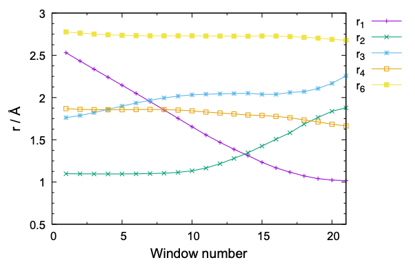
Note that 21 windows are set by the program. The number of window depends on the window interval, “-ds”. A large “ds” value reduces the number of window and the computational cost, yet with a higher risk that the neighboring windows have less or insufficient overlap of the probability distribution. The window interval of 0.1 Å with a force constant of 100 kcal/mol/Å2 is often used for chemical reactions. Nonetheless, it is always good to check the overlap in the initial equilibration steps, as we shall see in the next sub-section.
3. Equilibration 1
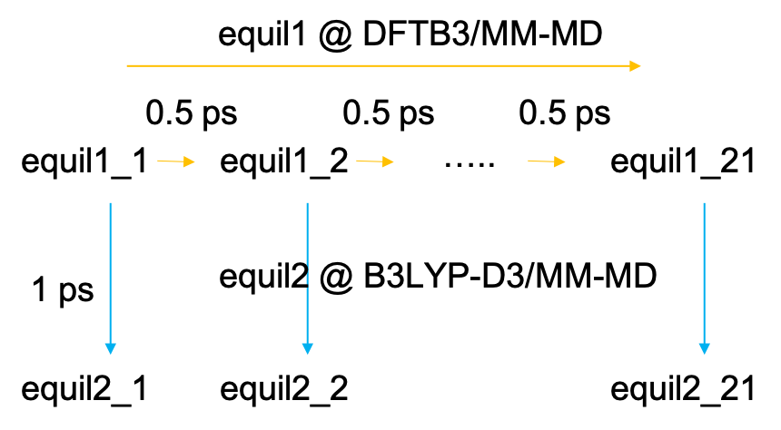
The equilibration MDs are done in two steps (Fig. 3). First, the MD is carried out sequentially starting from the first window to the last one. Each window is propagated for 500 fs at the level of DFTB3/MM. Then, in the next step, MDs of all windows (replicas) are carried out in parallel for 1 ps at the level of B3LYP-D3/MM.
Proceed to 1.equil,
$ cd 1.equil
$ ls
geninp1.sh   qsimulate.json   run.sh   template.inp   toppar
geninp1.sh is a script to generate input files of GENESIS for each
window based on a template file, template.inp. The template file is
shown below:
[INPUT]
topfile = toppar/top_all36_prot.rtf, toppar/top_all36_cgenff.rtf
parfile = toppar/par_all36_prot.prm, toppar/par_all36_cgenff.prm
strfile = toppar/toppar_water_ions.str, toppar/toppar_dhap.3.str
psffile = ../../2.equil/step4_nvt_100.psf     # protein structure file
pdbfile = ../../2.equil/step4_nvt_100.pdb     # PDB file
reffile = ../../2.equil/step4_nvt_100.pdb     # reference file
rstfile = ../../2.equil/step4.11_qmmm_nvt.rst # restart file

[OUTPUT]
dcdfile = equil1_ID.dcd
rstfile = equil1_ID.rst

[ENERGY]
forcefield       = CHARMM
electrostatic    = CUTOFF
switchdist       = 16.0      # switch distance
cutoffdist       = 18.0      # cutoff distance
pairlistdist     = 19.5      # pair-list distance
water_model      = NONE
vdw_force_switch = YES

[DYNAMICS]
integrator      = VVER
timestep        = 0.0005     # timestep (ps)
nsteps          = 1000       # number of MD steps
crdout_period   = 500
eneout_period   = 500
rstout_period   = 500
nbupdate_period = 10
stoptr_period   = 10
iseed           = 20190319

[CONSTRAINTS]
rigid_bond      = YES        # constraints all bonds involving hydrogen
shake_tolerance = 1.0D-10
hydrogen_type   = BOTH
fast_water      = YES
noshake_index   = 4 9 10 11  # don't constraint these hydrogen atoms

[ENSEMBLE]
ensemble        = NVT
tpcontrol       = BUSSI     # thermostat
temperature     = 300.0     # temperature (K)

[BOUNDARY]
type          = NOBC
spherical_pot = yes         # spherical potential

[QMMM]
qmtyp          = qsimulate       # QSimulate-QM
qmcnt          = qsimulate.json  # control file of QSimulate-QM
workdir        = equil1_ID
basename       = job
qmsave_period  = 500
qmmaxtrial     = 1
qmatm_select_index = 1
exclude_charge = group

[SELECTION]
group1  = sid:DHA or (sid:TIMA and (rno:95 or rno:165) and not (an:CA  | an:C   | an:O   | an:N | an:HN | an:HA))
group2  = atomno:1900 or atomno:5687 # COM of TIMA/TIMB
group3  = atomno:1442   # NE2 of HSE95
group4  = atomno:1443   # HE2 of HSE95
group5  = atomno:2559   # OE1 of GLU165
group6  = atomno:2560   # OE2 of GLU165
group7  = atomno:7584   # O2  of DHAP
group8  = atomno:7585   # C3  of DHAP
group9  = atomno:7587   # HO3 of DHAP
group10 = atomno:7588   # H31 of DHAP
group11 = atomno:7589   # H32 of DHAP


[RESTRAINTS]
nfunctions    = 6
function1     = POSI
constant1     = 10.0
select_index1 = 2

function2     = DIST    # r1(OE2-H31)
constant2     = 300.0
reference2    = R1
select_index2 = 6  10

function3     = DIST    # r2(C3-H31)
constant3     = 300.0
reference3    = R2
select_index3 = 8  10

function4     = DIST    # r3(OE1-HO3)
constant4     = 300.0
reference4    = R3
select_index4 = 5  9

function5     = DIST    # r4(O2-HE2)
constant5     = 300.0
reference5    = R4
select_index5 = 7   4

function6     = DIST    # r6(NE2-HO3)
constant6     = 300.0
reference6    = R5
select_index6 = 3  9
Note that:
- [INPUT]: The files in
2.equilare used to restart the job.rstfile=../../2.equil/step4.11_qmmm_nvt.rstis for the first window. Other windows restart from the previous window. - [OUTPUT], [QMMM]: “ID” is replaced by window ID.
- [ENERGY]: The switch and cutoff distances are longer than usual.
- [DYNAMICS]: The timestep is shorter than usual.
- [CONSTRAINTS]:
noshake_indexspecifies hydrogen atoms where SHAKE is disabled. The selection indicies 4, 9, 10, and 11 refer to HE2 of His95, HO3, H31, H32 of DHAP, respectively. - [QMMM]: QSimulate-QM is specified as a QM program.
qmexeis not needed, because GENESIS and QSimulate-QM are linked through dynamic libraries. - [SELECTION]: group1 is the QM region (DHAP and sidechain of His95 and Glu165), and group2-11 are used for the restraint.
- [RESTRAINTS]: The first function is a positional restraint of
the center of mass of TIMA and TIMB. Functions 2 – 6 are the
restraints of the atomic distances, r1 – r4 and r6,
respectively. R1, R2, …, R5 are replaced by the reference values
of each window.
qsimulate.jsonis a control file of QSimulate-QM. In this case, we use the DFTB3 method,
{ "bagel" : [

{
  "title" : "molecule",
  "basis" : "dftb" },
  {
    "title" : "force",
    "method" : [ {
      "title" : "dftb",
      "charge" : -3,
      "thresh" : 1.0e-5
    } ]
}

]}
Now, let’s run the script, geninp1.sh,
$ ./geninp1.sh
$ ls
equil1_1.inp    equil1_2.inp   equil1_3.inp  ...
equil1_xx.inp are input files of each window. Note that equil1_n.inp
restarts from equil1_(n-1).rst, as specified in rstfile of
[INPUT]. run.sh is a script to run the job,
#!/bin/bash
#
export LD_LIBRARY_PATH=/path/to/qsimulate/lib:$LD_LIBRARY_PATH  ... (1)
export PATH=$PATH:/path/to/genesis/bin                          ... (2)

export OMP_NUM_THREADS=4
export BAGEL_NUM_THREADS=${OMP_NUM_THREADS}
export MKL_NUM_THREADS=${OMP_NUM_THREADS}
export I_MPI_PERHOST=4
export I_MPI_DEBUG=5

nimg=$(wc ../0.window/win_rr.dat |awk '{print $1}')
for i in `seq 1 $nimg`; do
  mpiexec.hydra -n 2 atdyn equil1_${i}.inp >& equil1_${i}.out  ... (3)
done

exit 0
- Set the
LD_LIBRARY_PATHto where the dynamic libraries of QSimulate-QM are installed. - Set the
PATHto where GENESIS is installed. - Sequential run of equil1_1, equil1_2, … and equil1_nimg.
Now, run the job:
$ ./run.sh
4. Equilibration 2
When the job is done, proceed to 2.equil2,
$ cd ../2.equil2
$ ls
geninp2.sh   qsimulate.json   run.sh   template.inp   toppar
geninp2.sh generates an input file based on template.inp. The
template file is similar to before, but now there is [REMD]
section to run all windows (replicas) in parallel. We only show the
different parts below.
[INPUT]
...
rstfile = OLDNAME_{}.rst     # restart file

[OUTPUT]
logfile = NEWNAME_{}.log     # log file of each replica
dcdfile = NEWNAME_{}.dcd     # DCD trajectory file
remfile = NEWNAME_{}.rem     # parameter index file
rstfile = NEWNAME_{}.rst     # restart file

[REMD]
dimension         = 1           # dimension
exchange_period   = 0           # no exchange
type1             = RESTRAINT   # REUS
nreplica1         = NREP        # number of replicas
cyclic_params1    = NO          # Yes, if the parameter is periodic
rest_function1    = 2 3 4 5 6   # off-lattice REUS

[DYNAMICS]
integrator      = VVER
timestep        = 0.0005        # timestep (ps)
nsteps          = 2000          # 1 ps in total
crdout_period   = 20            # output for analysis
eneout_period   = 20
...

[ENSEMBLE]
...
tau_t           = 0.5   # accelerate the equilibration

[QMMM]
...
workdir        = NEWNAME
...

[RESTRAINTS]
nfunctions    = 6
...

function2     = DIST    # r1(OE2-H31)
constant2     = FC1
reference2    = R1
select_index2 = 6  10

...
- [INPUT], [OUTPUT], [QMMM]: NEWNAME and OLDNAME are basename of files. They are given by the arguments of
geninp2.sh(see below). - [REMD]
- exchange_period: The period of exchange attempt. No attempt is made when exchange_period=0.
- type1=RESTRAINT: Invokes REUS in the first dimension
- nreplica1: The number of replicas of the first dimension
- rest_function1: The restraint function used for REUS. Here, off-lattice REUS is invoked in which multiple restraints are merged into a single reaction coordinate.
- [DYNAMICS]: crdout_period and eneout_period are set to 20 to save the data for analyses.
- [ENSEMBLE]: tau_t = 0.5 is smaller than the default. This enables to equilibrate the system faster (~0.5 ps).
- [RESTRAINTS]: FC1 and R1 are replaced by the force constants and the reference distances of the windows (replicas).
qsimulate.json is a control file of QSimulate-QM, which now specifies
the B3LYP-D3/aug-cc-pVDZ level for DFT calculations. Refer to
tutorial-15.5 for details on the options.
Now, run geninp2.sh with NEWNAME and OLDNAME in the first and second
argument, respectively,
$ ./geninp2.sh equil2 ../1.equil1/equil1
$ ls
equil2_reus.inp   geninp.sh   qsimulate.json   run.sh
template.inp      toppar
euil2_reus.inp is the resulting input file. Note that the force
constants and the reference distances are written in a single line for
all windows:
$ grep -e constant2 -e reference2 equil2_reus.inp
constant2     =  100.0  100.0  ... 100.0  100.0
reference2    = 2.5300 2.4319  ...1.0232 1.0160
run.sh is a script to run the job,
$ cat run.sh
#!/bin/bash
#
export LD_LIBRARY_PATH=/path/to/qsimulate/lib:$LD_LIBRARY_PATH
export PATH=$PATH:/path/to/genesis/bin

export OMP_NUM_THREADS=4
export BAGEL_NUM_THREADS=${OMP_NUM_THREADS}
export MKL_NUM_THREADS=${OMP_NUM_THREADS}
export I_MPI_PERHOST=4
export I_MPI_DEBUG=5

mpiexec.hydra -n 168 atdyn equil2_reus.inp >& equil2_reus.out

exit 0
Here, we specify 8 MPI processes per replica, and request 8 MPI x 21 replicas = 168 MPI processes in total. Now we run the job,
$ ./run.sh
When the job is finished, it is a good point to do a sanity check before
the production run. Go to 2.equil2_analysis,
$ cd ../2.equil2_analysis
$ ls
analysis.sh        pathcv.inp         rmsd_analysis.inp
trj_analysis.inp   rst_convert.inp    ...
analysis.sh is a script to run analysis tools using the input files
shown above. Running the script yields an output for each window as
follow,
$ ./analysis.sh
1
2
.
.
21
$ ls
equil2_1.dis  equil2_1.pathcv  equil2_1.pdb  equil2_1.rms ...
Let us examine the results.
(1) Visualize the pdb files (the last snapshot of the trajectory) of each window,
$ vmd -e equil2.vmd
Make sure that the reaction takes place as intended and that there is nothing collapsing. For example, it happend to me before that the phosphate group left from DHAP. Unexpected weird (or perhaps interesting!) things can happen, so it is very important to visually check the structure.
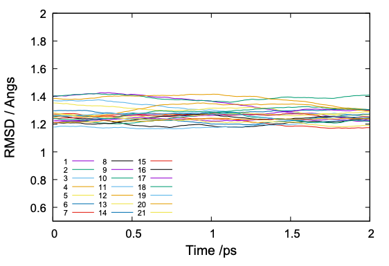
(2) Plot the RMSD of backbone heavy atoms of proteins,
$ gnuplot rmsd.gpi
The command plots RMSD of each replica and yields rmsd.pdf,
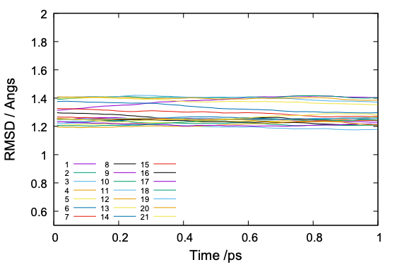
The value of RMSD is normally around 1 to 2. If the RMSD is much larger or abruptly changing along the simulation time, it is a sign that there is something happening in the protein structure.
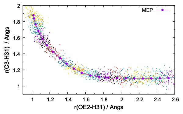
(3) Check the distribution.
$ gnuplot dist.gpi
$ gnuplot pathcv.gpi
The command gives the distribution of r~1~/r~2~ (dist.pdf), and the probability of pathCV 3 4 (pathcv.pdf and pathcv_all.pdf). The results are shown in Fig. 5.
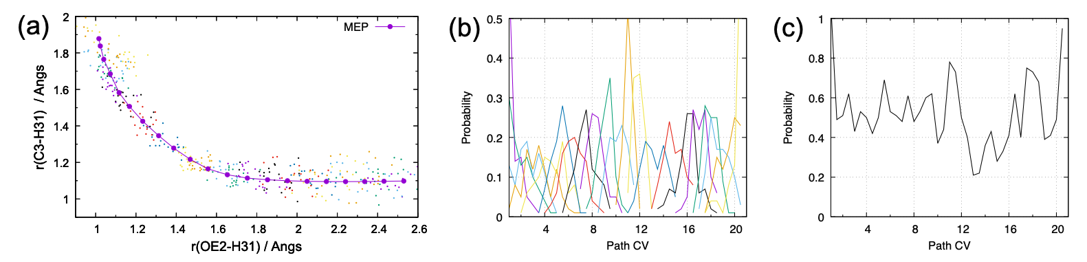
Although the number of sampling (100 points) is still few, these figures already tell that the distributions of each window are reasonably overlapped. One of the failure cases is that the distributions are much narrow and sharp, so that they have few overlap each other. In another case, the cumulative distribution exhibits a cleft, where the probability suddenly drops to zero. When the distribution is problematic, it is better to reset the parameters, i.e., add more windows and/or adjust the force constants, because longer simulation rarely solves the issue.
5. Production run
Now, we perform the production run. Proceed to 3.prod3,
$ cd ../3.prod3
$ ls
geninp2.sh   qsimulate.json   run.sh   template.inp   toppar
Again, we generate the input based on template.inp. It is almost the
same as the previous one except for [REMD] and [DYNAMICS] sections,
[REMD]
dimension         = 1
exchange_period   = 100    # attempt the exchange every 50 fs
...

[DYNAMICS]
integrator      = VVER
timestep        = 0.0005   # timestep (ps)
nsteps          = 2000     # 1 ps in total
crdout_period   = 10       # sample every 5 fs
eneout_period   = 10       # energy output period
rstout_period   = 100      # write restart
Most importantly, the replica exchange is attempted every 100 steps.
Note that mod(rstout_period, exchange_period) and
mod(nsteps,(2*exchange_period*dimension)) must be zero.
Now, generate the input and run the simulation,
$ ./geninp2.sh prod3 ../2.equil2/equil2
$ ls
geninp2.sh   prod3_reus.inp   qsimulate.json ...
$ ./run3.sh
This command carries out REUS MD simulations for 1 ps. It often happens that we want to extend the MD simulation. This can be done by,
$ ./geninp2.sh prod4 prod3
$ ls
geninp2.sh   prod4_reus.inp   qsimulate.json ...
$ ./run4.sh
prod4 restarts prod3 and extends the MD for another 1 ps. Note that
the length of MD can be adjusted by nsteps in the template file and
the number of jobs. For example, two jobs with nstep = 2000 is the
same as a single job with nstep = 4000. It is also possible to divide
the simulation into a smaller pieces. Such a flexibility is often useful
when the computational resources is busy.
When prod3 and prod4 are both finished, let us now analyze the
results. We first check the calculation. Proceed to 3.prod3_analysis,
$ cd ../3.prod3_analysis/
$ ls
acceptance_ratio.sh  prod4.vmd            replica_index.sh     rmsd_analysis.inp
analysis.sh          replica_index.gpi    rmsd_analysis.gpi    rst_convert.inp
(1) analysis.sh is a script to run rmsd_analysis and rst_convert for
each window. Running the script yields an output for each window as
follow,
$ ./analysis.sh
1
2
.
.
21
$ ls
prod4_1.pdb   prod4_1.rms ...
The pdb files can be visualized by VMD,
$ vmd -e prod4.vmd
and RMSD is plotted by gnuplot,
$ gnuplot rmsd_analysis.gpi
These results look reasonable. Nonetheless, we emphasize again that the sanity check is important to detect possible errors in the simulation.
(2) Given the output file of REUS, acceptance_ratio.sh yields the
acceptance ratio of each replica,
$ ./acceptance_ratio.sh ../3.prod3/prod4_reus.out
1 > 2 0.15
2 > 3 0.25
3 > 4 0.2
4 > 5 0.5
5 > 6 0.2
6 > 7 0.3
7 > 8 0.2
8 > 9 0.25
9 > 10 0.2
10 > 11 0.1
11 > 12 0.2
12 > 13 0.05
13 > 14 0.1
14 > 15 0.05
15 > 16 0.1
16 > 17 0.2
17 > 18 0.3
18 > 19 0.5
19 > 20 0.35
20 > 21 0.35
Although there are several replicas with low acceptance ratio, most replicas show an acceptance ratio of 0.2 – 0.3.
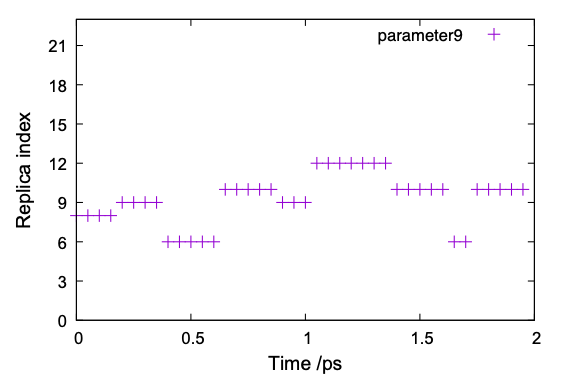
(3) Let us also check the time course of the index of replica.
$ ./replica_index.sh
$ gnuplot replica_index.gpi
The result of one of the parameters (parameter 9) is shown in Fig. 7. It is observed that parameter 9 is exchanged among replica ID 6 – 12, but not in the whole space. A similar tendency is observed in other replicas as well, suggesting that the MD simulation needs to extend to achieve random walk in the replica space.
6. The potential of mean-force (PMF)
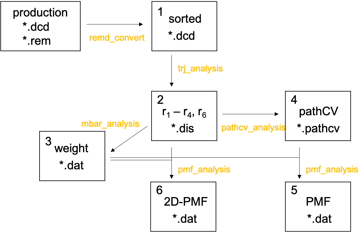
Now, we calculate the PMF along the reaction path. Proceed to 4.pmf
and find six sub-directories,
$ cd ../4.pmf
$ ls
1.sort_dcd/    2.calc_dist/   3.mbar/
4.calc_pathcv/ 5.pmf_pathcv/  6.pmf_r1r2/
For clarity, the procedure is outlined in Fig. 8, where the number in the box corresponds to the number of the directories. Also, the analysis tools used in each step are shown in yellow text.
The script to run the analysis tools, run.sh, are prepared in all
directories,
$ ls */run.sh
1.sort_dcd/run.sh   3.mbar/run.sh         5.pmf_pathcv/run.sh
2.calc_dist/run.sh  4.calc_pathcv/run.sh  6.pmf_r1r2/run.sh
These files start with the following lines,
#!/bin/bash

export PATH=${PATH}:/path/to/genesis/bin
Change “/path/to” to the directory where GENESIS is installed.
6.1. Sort DCD
Because the REUS simulation prints the coordinates (dcd files) in terms of replica ID, we first sort the coordinates in terms of parameter ID. Proceed to 1.sort_dcd,
$ cd 1.sort_dcd
$ ls
remd_convert3.inp  remd_convert4.inp  run.sh
remd_convert3.inp is an input file of remd_convert, which is shown
below,
[INPUT]
reffile = ../../../2.equil/step4_nvt_100.pdb
dcdfile = ../../3.prod3/prod3_{}.dcd
remfile = ../../3.prod3/prod3_{}.rem   # REMD parameter ID file
logfile = ../../3.prod3/prod3_{}.log   # REMD energy log file

[OUTPUT]
pdbfile = prod3_param.pdb        # PDB file
trjfile = prod3_param{}.dcd      # trajectory file
logfile = prod3_param{}.log      # REMD energy log file

[SELECTION]
group1         = all

[FITTING]
fitting_method = NO

[OPTION]
convert_type    = PARAMETER      # (REPLICA/PARAMETER)
num_replicas    = 21             # total number of replicas
nsteps          = 2000           # nsteps in [DYNAMICS]
exchange_period = 100            # exchange_period in [REMD]
crdout_period   = 10             # crdout_period in [DYNAMICS]
eneout_period   = 10             # eneout_period in [DYNAMICS]
trjout_format   = DCD            # (PDB/DCD)
trjout_type     = COOR           # (COOR/COOR+BOX)
trjout_atom     = 1              # atom group
centering       = NO             # shift center of mass
pbc_correct     = NO             # (NO/MOLECULE)
remd_convert reads the parameter ID from remfile, and sorts the
coordinates in terms of parameter ID with covert_type = PARAMETER.
remd_convert4.inp converts the dcd files of prod4 in the same way.
run.sh reads,
remd_convert remd_convert3.inp >& remd_convert3.out
remd_convert remd_convert4.inp >& remd_convert4.out
Now, run the script,
$ ./run.sh
$ ls
prod3_param1.dcd   prod3_param1.log ...
prod4_param1.dcd   prod4_param1.log ...
The new dcd files, prod[3,4]_parmID.dcd, contain the coordinates of
the parameter ID. The energies are sorted similarly and written in the
log files, though they are not used in the current analysis.
6.2. Calculate distance
Proceed to 2.calc_dist,
$ cd ../2.calc_dist
$ ls
dist.gpi    run.sh    trj_analysis.inp
trj_analysis.inp is an input file of trj_analysis, which calculates
the distances, r1 – r4 and r6, from dcd files.
[INPUT]
psffile = ../../../2.equil/step4_nvt_100.psf
reffile = ../../../2.equil/step4_nvt_100.pdb

[OUTPUT]
disfile        = prod3_NUM.dis      # distance file

[TRAJECTORY]
trjfile1       = ../1.sort_dcd/prod3_paramNUM.dcd     # trajectory file
trjfile2       = ../1.sort_dcd/prod4_paramNUM.dcd     # trajectory file
md_step1       = 200             # number of MD steps
mdout_period1  = 1               # MD output period
ana_period1    = 1               # analysis period
repeat1        = 2               # the number of repeat
trj_format     = DCD             # (PDB/DCD)
trj_type       = COOR            # (COOR/COOR+BOX)
trj_natom      = 0

[OPTION]
check_only     = NO
allow_backup   = NO
distance1      = TIMA:165:GLU:OE2 DHA:249:DHAP:H31 # r1 (OE2 - H31)
distance2      = DHA:249:DHAP:C3  DHA:249:DHAP:H31 # r2 (C3  - H31)
distance3      = TIMA:165:GLU:OE1 DHA:249:DHAP:HO3 # r3 (OE1 - HO3)
distance4      = DHA:249:DHAP:O2  TIMA:95:HSE:HE2  # r4 (O2  - HE2)
distance5      = TIMA:95:HSE:NE2  DHA:249:DHAP:HO3 # r6 (NE2 - HO3)
“NUM” is replaced by the parameter ID at runtime in run.sh. Note that
the dcd files of prod3 and prod4 are read at the same time
(repeat = 2) and that all the data (400 points) are printed to
prod3_NUM.dis.
Now, run the script,
$ ./run.sh
$ ls
dist.gpi   prod3_1.dis   prod3_2.dis   ...
dist.gpi plots the distribution of r1 / r2,
$ gnuplot dist.gpi
6.3 MBAR
Here, we solve the MBAR equation 5 and obtain the weight of each
snapshot. Proceed to 3.mbar,
$ cd ../3.mbar
$ ls
mbar.inp  run.sh
mbar.inp is an input file of mbar_analysis,
[INPUT]
cvfile = ../2.calc_dist/prod3_{}.dis   # distant files

[OUTPUT]
fenefile       = fene.dat       # free energy file
weightfile     = weight{}.dat   # weight file

[MBAR]
dimension          = 1
num_replicas       = 21
input_type         = US         # Umbrella sampling
tolerance          = 10E-08     # threshold of MBAR iteration
temperature        = 300.0      # simulation temperature
target_temperature = 300.0      # target temperature
rest_function1     = 1 2 3 4 5  # r1 - r4, r6

nblocks          = 1
self_iteration   = 5
Newton_iteration = 40

[RESTRAINTS]
constant1     =  100.0  100.0  100.0  ...  100.0 # r1 (OE2 - H31)
reference1    = 2.5300 2.4319 2.3358  ... 1.0160
...

is_periodic1 = no
...
run.sh reads,
export OMP_NUM_THREADS=4
mbar_analysis mbar.inp >& mbar.out
mbar_analysis is thread-parallelized, and setting the variable,
OMP_NUM_THREADS, accelerates the calculation. Now, run the script,
$ ./run.sh
$ ls
fene.dat   weight1.dat   weight2.dat ...
weightID.dat contains the weight of trajectory snapshots for each
parameter ID. Using the weight, we can readily calculate the
thermodynamic average of any quantity. In the following subsections, 1D-
and 2D-PMFs are calculated in terms of pathCV and r~1~/r~2~,
respectively.
6.4 1D-PMF along pathCV
Now, proceed to 4.calc_pathcv,
$ cd ../4.calc_pathcv
$ ls
pathcv.gpi  pathdist.gpi   pathcv.inp  run.sh
pathcv.inp is an input file of pathcv_analysis.
[INPUT]
pathfile = ../../0.window/win_rr.dat    # the information of discretized path
cvfile   = ../2.calc_dist/prod3_{}.dis  # CV data

[OUTPUT]
pathcvfile = prod3_{}.pathcv  # pathCV and distance

[OPTION]
nreplica   = 21
PathCV 3 represents the reaction coordinate by discrete points and
enumerates them from 1 to N (N is the number of points). Here, the
discrete points are set to the anchor points of US, given by pathfile.
Then, the program calculates for each data points given by cvfile the
pathCV and path distant, which indicate where in the path the point is
ascribed to and how distant it is from the path, respectively.
Now, run the script,
$ ./run.sh
$ ls
pathcv.inp  pathcv.out  prod3_1.pathcv   prod3_2.pathcv ...
The pathCV and distance are printed in the second and third columns of
prod3_x.pathcv, respectively. These values are plotted by,
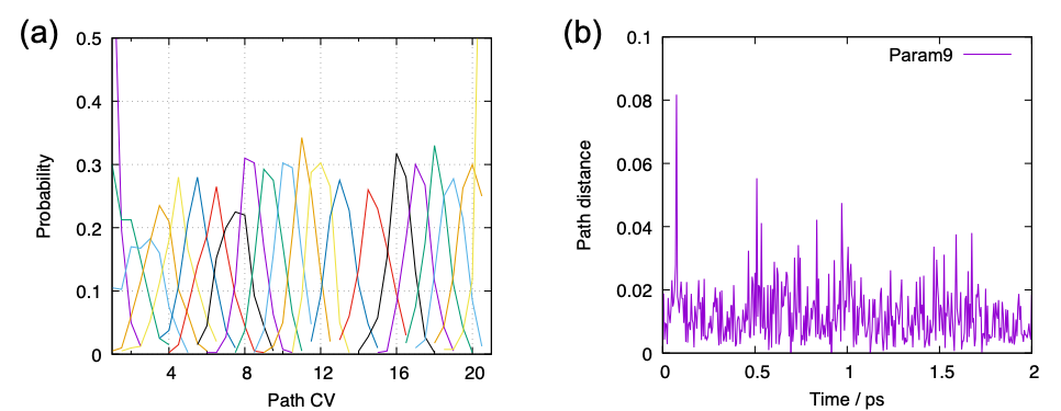
$ gnuplot pathcv.gpi
$ gnuplot pathdist.gpi
The first line yields Fig. 10 (a). The probability distribution of each parameter has sufficient overlap in terms of pathCV. The second line plots the time course of the path distance of all parameters in a big sheet; here we show only one of them, parameter 9, in Fig. 10 (b). Although the path distance is around 0.01 – 0.02 on average, the trajectory largely deviates from the path in some occations. Since such occational large deviation cause numerical errors, it is recommended to set a cutoff that is 2 – 3 times larger than the average value when calculating the PMF. We use cutoff=0.04 below.
Proceed to 5.pmf_pathcv,
$ cd ../5.pmf_pathcv
$ ls
pmf.gpi   pmf_bw15.inp  pmf_bw20.inp  run.sh
pmf_bw*.in are the input file of pmf_analysis.
[INPUT]
weightfile     = ../3.mbar/weight{}.dat             # weight file
cvfile         = ../4.calc_pathcv/prod3_{}.pathcv   # pathCV
distfile       = {}.pathdist                        # path distance

[OUTPUT]
pmffile        = pmf_bw15.dat    # potential of mean force

[OPTION]
nreplica       = 21
dimension      = 1
temperature    = 300
cutoff         = 0.04          # cutoff distance
grids1         = 1.0 21.0 101  # (min max num_of_bins)
band_width1    = 0.15          # sigma of Gaussian kernel
is_periodic1   = NO
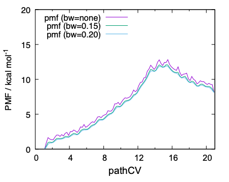
cutoff is set to 0.04 based on the result in Fig. 10 (b). In
pmf_analysis, Gaussian kernel is used to smoothen the PMF, and the
bandwidth of the Gaussian function is specified by band_width1.
Although the smoothening is useful to reduce the noise, the bandwidth
should be carefuly chosen so as to not to incurr any artifact. The
bandwidth is set to 0.15 and 0.20 in pmf_dat15.inp and
pmf_dat20.inp, respectively.
Now, run the job,
$ ./run.sh
$ ls
pmf_bw15.dat   pmf_bw15.inp   pmf_bw15.out
pmf_bw20.dat   pmf_bw20.inp   pmf_bw20.out  ...
dat files contain the PMF along pathCV with and without the Gaussian smoothing. Finally, the data is plot by gnuplot,
$ gnuplot pmf.gpi
$ ls
pmf.gpi   pmf.pdf   pmf_bw15.dat ...
6.5. 2D-PMF in r1/r2
Let us calculate a 2-dimensional (2D) PMF as a function of r~1~ and
r~2~. Since r~1~ and r~2~ are already obtained for each snapshots in
2.calc_dist, we go directly to pmf_analysis. Proceed to
6.pmf_r1r2,
$ cd ../6.pmf_r1r2
$ ls
2dsurf_mix.gpi   pmf.inp   run.sh
pmf.inp is an input file,
[INPUT]
weightfile     = ../3.mbar/weight{}.dat       # weight file
cvfile         = ../2.calc_dist/prod3_{}.dis  # r1 and r2

[OUTPUT]
pmffile        = pmf2.dat      # potential of mean force

[OPTION]
nreplica       = 21
dimension      = 2             # 2D-PMF
temperature    = 300
output_type    = GNUPLOT       # print the output in gnuplot style

grids1         = 0.8 2.8 101   # (min max num_of_bins)
band_width1    = 0.020         # sigma of Gaussian kernel
is_periodic1   = NO

grids2         = 0.9 2.4 101   # (min max num_of_bins)
band_width2    = 0.020         # sigma of Gaussian kernel
is_periodic2   = NO
The dimension is set to 2, and the gridsX, band_widthX, is_periodicX
(X=1,2) are set for the first and second dimensions, i.e., r1 and
r2, respectively. Note that r1 and r2 are written in the second
and third columns of prod3_*.dis, respectively, and thus we can use
them as is for cvfile.
Now, run the script,
$ ./run.sh
$ ls
pmf.inp      pmf.out      pmf2.dat ...
pmf2.dat contains the data of 2D-PMF in a gnuplot format. Finally, plot
the data using gnuplot,
$ gnuplot 2dsurf_mix.gpi
$ ls
2dsurf_mix.gpi  2dsurf_mix.pdf  pmf.inp ...
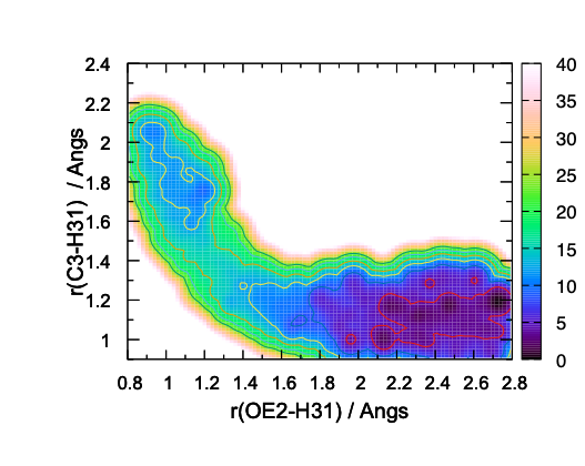
The resulting 2D-PMF in Fig. 12 shows the overall shape of the free-energy landscape. However, some contour lines (4 and 8 kcal/mol, in particular) show wiggle shape, which is an indication of insufficient sampling.
7. Concluding remarks
We have demonstrated REUS simulations with a QM/MM potential using GENESIS/QSimulate-QM for calculating the free-energy landscape of an enzymatic reaction. 1D- and 2D-PMF have been calculated in terms of pathCV and r~1~/r~2~, respectively, using the MBAR method.
QM/MM-MD simulations have been performed for 2 ps per replica, thereby 2 x 21 = 42 ps in total. The resulting PMF along pathCV is found to be reasonably converged, yielding a barrier height of ~ 12 kcal/mol. On the other hand, the 2D-PMF in terms of r~1~/r~2~ has turned out to be insufficient in the number of sampling.
One of the main issues of REUS with QM/MM-MD is the high computational cost. The number of QM calculations is 6000 points x 21 replica = 126,000 points in this tutorial, and it could be even more in real applications. Therefore, fast QM programs with rich computational resource is a key technical element, e.g., QSimulate-QM with supercomputers, TeraChem with GPGPU clusters, and so on. On the other hand, utilizing the semiempirical methods such as DFTB is another promising direction, since DFTB is orders of magnitude cheaper than DFT (see 1.equil1 vs 2.equil2). For example, one may perform MD simulations with DFTB and reweight the energy landscape to DFT level. Such a multi-level approch will be our next goal.
Written by Kiyoshi Yagi@RIKEN Theoretical molecular science laboratory
April., 3, 2022
References
-
Y. Sugita, A. Kitao, and Y. Okamoto, J. Chem. Phys. 113, 6042-6051 (2000). ↩
-
K. Yagi, S. Ito, and Y. Sugita, J. Phys. Chem. B 125, 4701-4713 (2021). ↩
-
D. Branduardi, F. L. Gervasio, M. Parrinello, J. Chem. Phys. 126, 054103 (2007). ↩ ↩2
-
Y. Matsunaga, Y. Komuro, C. Kobayashi, J. Jung, T. Mori, and Y. Sugita, J. Phys. Chem. Lett. 7, 1446−1451 (2016). ↩
-
M. R. Shirts and J. D. Chodera, J. Chem. Phys. 129, 124105 (2008). ↩