GENESIS Tutorial 14.2 (2022)

Absolute solvation free energy

0. Preparations

All the files required for this tutorial are hosted in the [GENESIS tutorials repository on GitHub] (https://github.com/genesis-release-r-ccs/genesis_tutorial_materials). If you haven’t downloaded the files yet, open your terminal and run the following command (see more in Tutorial 1.1):

$ cd ~/GENESIS_Tutorials-2022
# if not yet
$ git clone https://github.com/genesis-release-r-ccs/genesis_tutorial_materials

If you already have the tutorial materials, let’s go to our working directory:

$ cd genesis_tutorial_materials/tutorial-14.2

1. Alchemical calculation for absolute solvation free energy

The absolute solvation free energy, \(\Delta G_{\rm solv}\), is the free-energy change upon the transfer of a solute from vacuum to solvent. In Figure 1, we can see that the calculation of the absolute solvation free energy is a special case of the relative solvation free energy calculation (Figure 2 in Sec. 14.1), where molecule B is nothing. Molecule B has the same topology and force field parameters as molecule A, but the interactions of molecule B with the solvent molecules are turned off (i.e., fully decoupled from the system). The free-energy change from fully interacted state (molecule A) to fully decoupled state (molecule B), \(\Delta G_{\rm annih}^{\rm vacuum}\) and \(\Delta G_{\rm annih}^{\rm solvent}\), can be calculated by gradually annihilating the interactions of the solute in vacuum and in solvent, respectively. Thus, \(\Delta G_{\rm solv}\) can be calculated via the alchemical calculation paths (Figure 1):

\[ \begin{aligned} \Delta G_{\rm solv} = \Delta G_{\rm annih}^{\rm vacuum} + \Delta G_{\rm tr} -- \Delta G_{\rm annih}^{\rm solvent}, \end{aligned} \]

where \(\Delta G_{\rm tr}\) is the change in the free energy of translational and rotational motion of the solute. In the fully decoupled state (molecule B), the solute can move freely in the simulation box both in vacuum and in solvent, resulting in \(\Delta G_{\rm tr}=0\). In this tutorial, we will demonstrate how to calculate \(\Delta G_{\rm annih}^{\rm vacuum}\) and \(\Delta G_{\rm annih}^{\rm solvent}\) using the FEP functions in GENESIS.

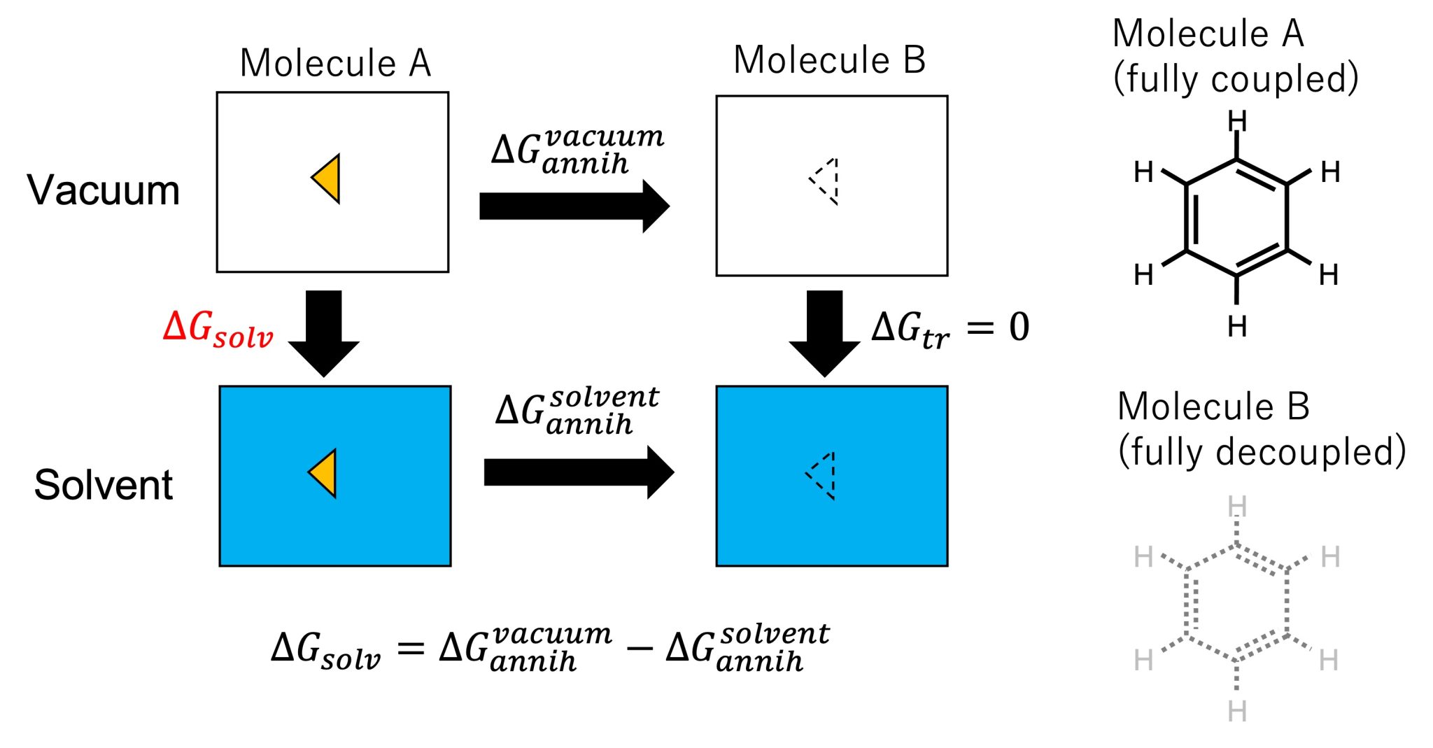
Figure 1. (Left) Thermodynamic cycle for calculating solvation free energy and annihilation of the solute. (Right) Molecules A and B.

2. System setup

2. 1. Overview of required input files

In this tutorial, we demonstrate the alchemical calculation of the absolute solvation free energy for methane and methanol. The tutorial consists of three directories: methane, methanol, and toppar. The “methane” and “methanol” directories include “ligand and vacuum directories, which contain input files for FEP simulations in solvent and in vacuum, respectively. The “toppar directory contains CHRAMM force field parameter files.

# Download the tutorial file
$ cd tutorial-14.2
$ ls
methane/  methanol/  toppar/
$ cd methane
$ ls
calc_dG.py  ligand/  README  vacuum/

# Setup the directory for binary files of GENESIS 2.1.X
$ export GENESIS_BIN_DIR=../../../GENESIS_Tutorials-2022/Programs/genesis-2.1.X/bin/

The ligand directory contains script files and input files for calculating \(\Delta G_{\rm annih}^{\rm solvent}\). run_min.inp, run_eq1.inp, run_eq2.inp, and run_eq3.inp are GENESIS control files for minimization, heating, equilibration with restraints, and equilibration without restraints, respectively. make_inp.sh is a shell script for generating the control file for the production run of FEP simulations. post_run.sh is a shell script for analysis. The vacuum directory contains respective input files for calculating of \(\Delta G_{\rm annih}^{\rm vacuum}\).

$ cd ligand
$ ls
run_eq.sh*      ligand.psf      output/         run_eq2.inp     run_fep2.inp
run_fepremd.sh* make_input.sh*  post_run.sh*    run_eq3.inp     run_min.inp
ligand.pdb      make_job.sh*    run_eq1.inp     run_fep1.inp

2. 2. Structure files for the hybrid-topology approach

Unlike the relative solvation free energy calculations, in the absolute solvation case, there is no target molecule (molecule B), i.e. the single-topology part is nothing, thus there are no atoms corresponding to singleA and singleB. Therefore, we do not use the hybrid topology setup. We consider the solute as having only the dual-topology part where dualA corresponds to the fully coupled solute, while dualB corresponds to “nothing” (i.e., the solute has fully disappeared from the system). Figure 2 shows a section of the PDB file, which contains only the coordinates of the solute (methane) corresponding to dualA, and solvent molecules. It does not include a dualB part, because the target state (state B) does not have any solute.

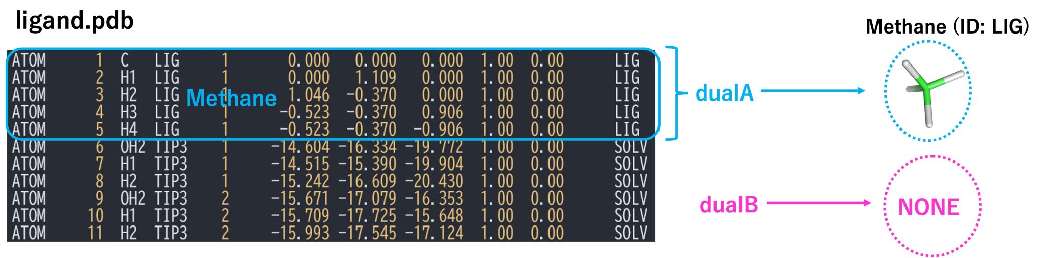
Figure 2. PDB file for the dual topology and definitions of dualA, and dualB.

The input files in tutorial-14.2.zip were generated by CHARMM-GUI Absolute Ligand Solvator, but some files were modified for the purpose of this tutorial.

3. FEP simulations in solvent

3. 1. Minimization and equilibration

We carry out minimization and equilibration of the system. As shown in Figure 2, the system has only one solute, therefore we do not need special treatment for overlaps or superimposition of molecules A and B. We perform minimization and equilibration similarly to conventional MD simulations, the [ALCHEMY] section is not included in run_min.inp, run_eq1.inp, run_eq2.inp, and run_eq3.inp.

First, we carry out the minimization in order to remove atomic clashes in the initial structure. The following command executes the minimization procedure:

# Perform minimization
$ $GENESIS_BIN_DIR/spdyn -np 8 run_min.inp > output/run_min.out

Next, we heat up the system from 0.1 K to 300 K. The following command executes the heating procedure:

# Perform heating
$ $GENESIS_BIN_DIR/spdyn -np 8 run_eq1.inp > output/run_eq1.out

Subsequently, we perform NPT equilibration with restraints (100 ps) and NPT equilibration without restraints (100 ps). In those simulations, [ALCHEMY] is the same as the heating. After the simulations have ended, it is recommended to check the log files and confirm the trajectories using a visualization tool such as VMD.

# Perform equilibration with positional restraints
$ $GENESIS_BIN_DIR/spdyn -np 8 input/run_eq2.inp > output/run_eq2.out

# Perform equilibration without the restraints
$ $GENESIS_BIN_DIR/spdyn -np 8 input/run_eq3.inp > output/run_eq3.out

3. 2. FEP/\(\lambda\) REMD simulations

In this step, we perform the production run of FEP/REMD simulations. We prepare 24 replicas: The first and the last replicas correspond to the initial and final states, respectively, while the other 22 replicas correspond to intermediate states. 24 replicas run in parallel and exchange their parameters at fixed intervals during the simulation. Exchanges between adjacent replicas are accepted or rejected according to the Metropolis criterion ¹,².

We execute two 1-ns FEP/REMD simulations (run_fep1.inp and run_fep2.inp) sequientially for a total of a 2-ns simulation. Input files for sequential runs can be easily generated by the following command:

# Execute the shell script for generation of input files
$ sh make_inp.sh

The simulation time can be modified in the “make_inp.sh” script (5-ns by default). If 24 replicas are too large for the user’s computer resources, it is recommended to use the “embarrassingly parallel computing” option by modifying make_inp.sh (see Sec 14.1.6).

The most important sections in run_fep1.inp are shown below. In the FEP/REMD simulation, [REMD] section is also required. type1 is set to alchemy, meaning that \(\lambda\) values are exchanged. exchange_period should be a multiple of fepout_period. nreplica1 specifies the number of replicas. In the [ALCHEMY] section, fep_direction is set to Bothsides. Figure 3 shows the fepfile file for replica 1 (= window 1). The fepfile files are used to calculate the free energy in the next section “4. Analysis”. Here we use the dual-topology approach, “fep_topology = [dual]”. Since there are no single-topology parts, singleA and singleB are set to NONE. dualA is set to the group ID specified in the [SELECTION] section, while dualB is set to NONE. This specifies that there is no target state (molecule B is nothing) and only the interactions of molecule A are scaled according to the \(\lambda\) values. The parameters for LJ and electrostatic soft-core potentials ³,⁴ are set to 5.0 and 0.5, respectively (sc_alpha=5.0 and sc_beta=0.5). The parameters for specifying \(\lambda\) values for each replica are lambljA, lambljB, lambelA, lambelB, lambbondA, lambbondB, and lambrest, but in this case only lambljA and lambelA are used (lambljB, lambelB, lambbondA, lambbondB, and lambrest can have any values). As shown in Figure 4, we start by linearly changing lambelA from 1.0 to 0.0 (replica 1 to replica 11). After annihilating the electrostatic interactions, we gradually change lambljA from 1.0 to 0.0 (replica 12 to replica 24). Since the energy difference often becomes very large near lambljA = 0, more intermediate states should be inserted in order to reduce statistical errors.

[REMD]
dimension = 1
exchange_period = 800
type1 = alchemy
nreplica1 = 24

[ALCHEMY]
fep_direction = BothSides
fep_topology = dual
singleA = NONE
singleB = NONE
dualA   = 1
dualB   = NONE
fepout_period = 400
equilsteps = 0
sc_alpha   = 5.0
sc_beta    = 0.5
lambljA       = 1.000 1.000 1.000 1.000 1.000 1.000 1.000 1.000 1.000 1.000 \
                1.000 0.900 0.800 0.700 0.600 0.500 0.400 0.300 0.200 0.150 \
                0.100 0.050 0.025 0.000
lambljB       = 0.000 0.000 0.000 0.000 0.000 0.000 0.000 0.000 0.000 0.000 \
                0.000 0.000 0.000 0.000 0.000 0.000 0.000 0.000 0.000 0.000 \
                0.000 0.000 0.000 0.000
lambelA       = 1.000 0.900 0.800 0.700 0.600 0.500 0.400 0.300 0.200 0.100 \
                0.000 0.000 0.000 0.000 0.000 0.000 0.000 0.000 0.000 0.000 \
                0.000 0.000 0.000 0.000
lambelB       = 0.000 0.000 0.000 0.000 0.000 0.000 0.000 0.000 0.000 0.000 \
                0.000 0.000 0.000 0.000 0.000 0.000 0.000 0.000 0.000 0.000 \
                0.000 0.000 0.000 0.000
lambbondA     = 1.000 1.000 1.000 1.000 1.000 1.000 1.000 1.000 1.000 1.000 \
                1.000 1.000 1.000 1.000 1.000 1.000 1.000 1.000 1.000 1.000 \
                1.000 1.000 1.000 1.000
lambbondB     = 0.000 0.000 0.000 0.000 0.000 0.000 0.000 0.000 0.000 0.000 \
                0.000 0.000 0.000 0.000 0.000 0.000 0.000 0.000 0.000 0.000 \
                0.000 0.000 0.000 0.000
lambrest      = 1.000 1.000 1.000 1.000 1.000 1.000 1.000 1.000 1.000 1.000 \
                1.000 1.000 1.000 1.000 1.000 1.000 1.000 1.000 1.000 1.000 \
                1.000 1.000 1.000 1.000

[SELECTION]
group1 = segid:LIG

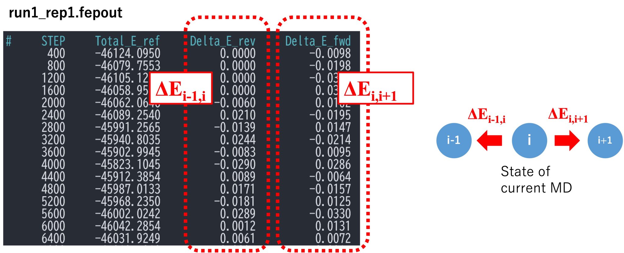
Figure 3. A section of fepfile file.

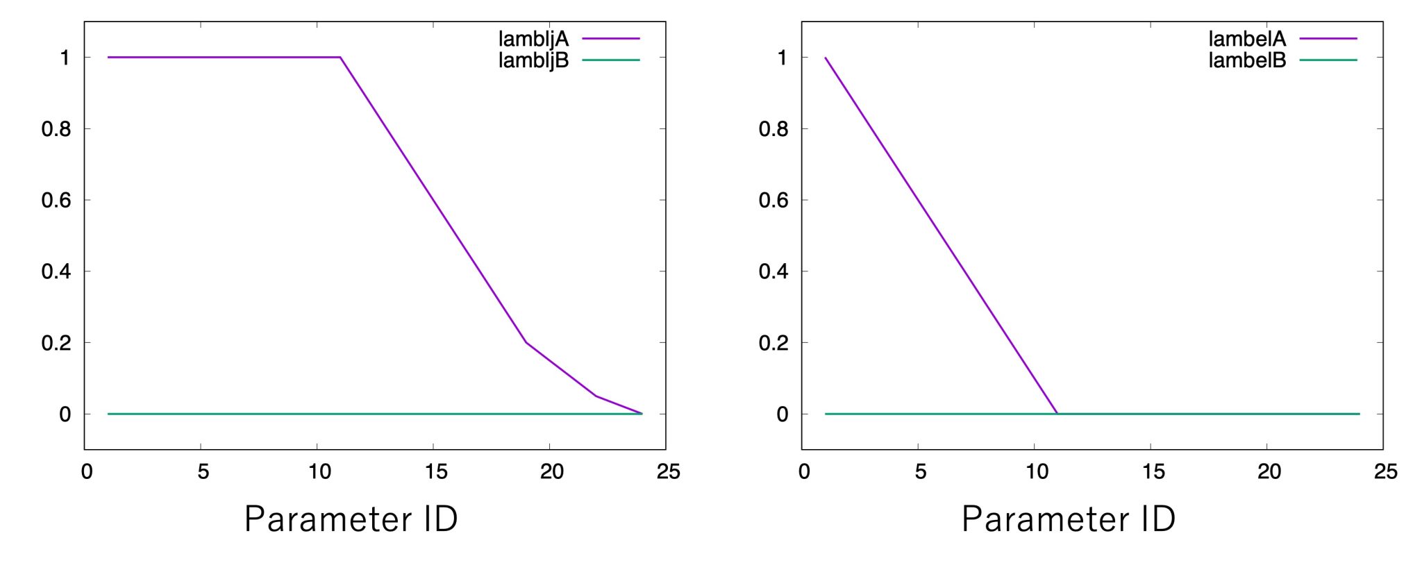
Figure 4. Values of λ for electrostatic and LJ interactions.

The following command executes the FEP/\(\lambda\)REMD simulation:

# Execute the control file for the lambda-exchange FEP simulation
# 8 MPI processes per replica, i.e. 8 * 24 = 192 processes are used here
$ $GENESIS_BIN_DIR/spdyn -np 192 input/run_fep1.inp > output/run_fep1.out

We perform a FEP/\(\lambda\)REMD simulation using the r-RESPA integrator with a 2.5-fs time step. Here, the length of the simulation is 2 ns, which might not be sufficient for the convergence of the free-energy calculation. For obtaining more accurate results, it is recommended to use a longer simulation time, in accordance with the computational resources or time available for the user.

3. 3. Analysis

After the FEP/\(\lambda\)REMD simulations have ended, we calculate the free energy from the fepfile files. The post_run.sh script calculates the free-energy difference between the initial and final states:

# Execute the shell script for analysis
$ sh post_run.sh

In the first part of the post_run.sh script, fepfile files are sorted using remd_convert and energy differences for each parameter are outputted (par1.fepout to par24.fepout). After sorting, the free-energy differences between the reference state (state A = fully coupled) and the target state (state B = fully decoupled) are calculated using mbar_analysis in GENESIS analysis tool. Finally, post_run.sh outputs a file named fene.dat (Figure 5). By default, the trajectories are divided into three blocks, and each column in fene.dat represents the free-energy changes in each block (i.e., the block average of the free-energy changes are obtained). Each row represents the free-energy change from the initial state (state A). The last row corresponds to the free-energy change from the initial state to the final state (state B), which is equal to \(\Delta G_{\rm annih}^{\rm solvent}\).

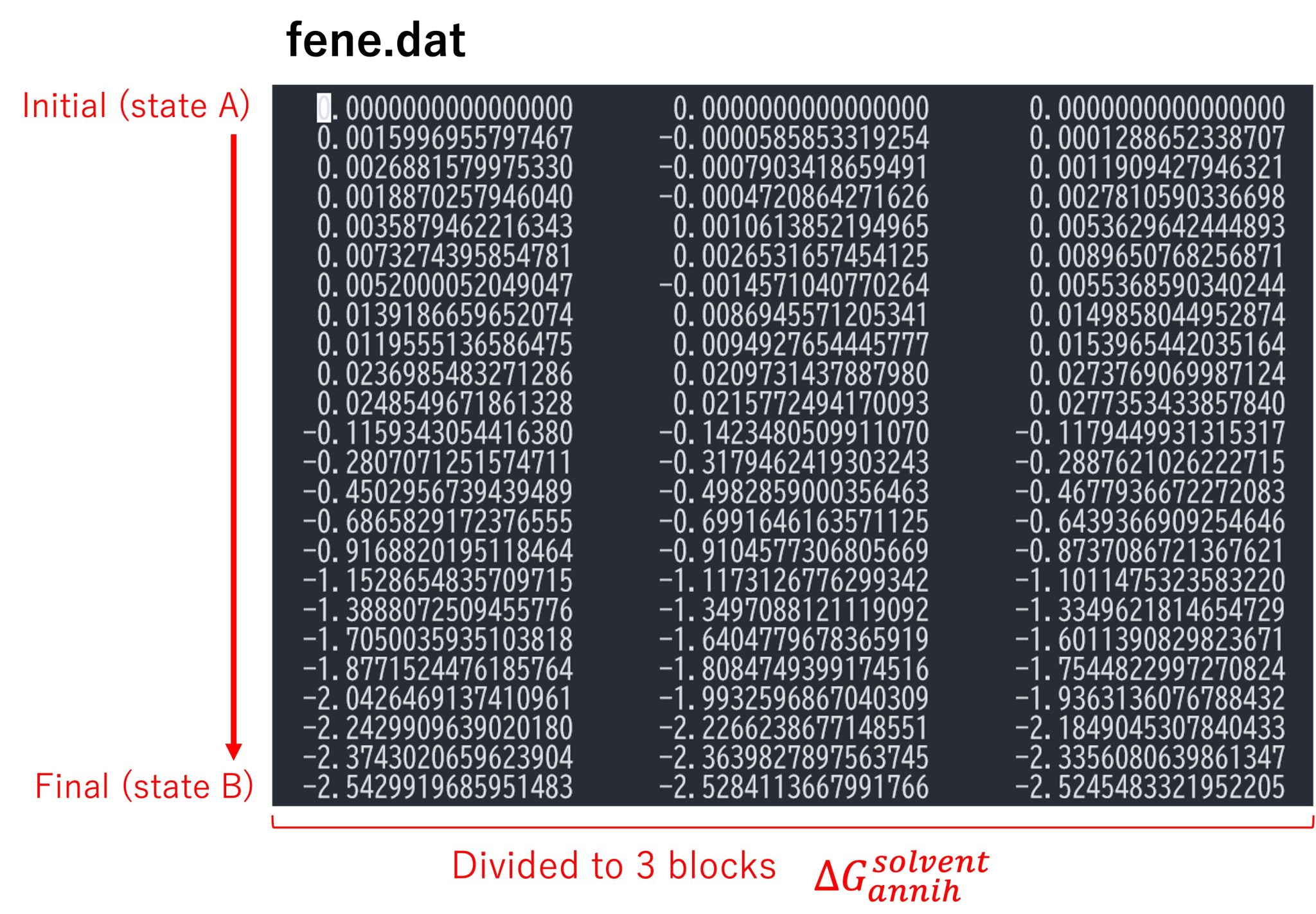
Figure 5. Free-energy changes from the initial state to the final state in the solvent.

4. FEP simulations in vacuum

Next, we perform FEP simulations in vacuum to obtain \(\Delta G_{\rm annih}^{\rm vacuum}\) . Please change directory to vacuum. Input files for the vacuum simulations are very similar to those for the solvent simulations, but there are some important differences described as follows. There are no water molecules in vacuum.pdb and vacuum.psf. In run_min.inp, run_eq[1-3].inp, and run_fep[1-2].inp, vacuum option is set to “YES”. CUTOFF is used for energy evaluation instead of PME. The cutoff distance should be set to a sufficiently large value (here we use 300 Å). The box size should be consistent with the large pairlist distance. Also, NVT should be used in order to fix the simulation box size. If NPT is used in the vacuum simulation, the box size shrinks drastically, which can lead to an early termination of the simulation.

[ENERGY]
forcefield       = CHARMM       # [CHARMM]
electrostatic    = CUTOFF       # [CUTOFF,PME]
switchdist       = 298.0        # switch distance
cutoffdist       = 300.0        # cutoff distance
pairlistdist     = 305.0        # pair-list distance
vdw_force_switch = YES
vacuum           = YES

[BOUNDARY]
type            = PBC           # [PBC]
box_size_x      = 921
box_size_y      = 921
box_size_z      = 921

Similarly to FEP simulations in solvent, after performing minimization, equilibration, and FEP/\(\lambda\)REMD simulations, we can obtain \(\Delta G_{\rm annih}^{\rm vacuum}\) by executing post_run.sh.

5. Calculation of \(\Delta G_{\rm solv} \) and \(\Delta\Delta G_{\rm solv} \) and comparison with experimental values

Figure 6 shows the free-energy changes of methane and methanol. The free-energy changes in window ID 24 for “in solvent” and “in vacuum” correspond to \(\Delta G_{\rm annih}^{\rm solvent}\) and \(\Delta G_{\rm annih}^{\rm vacuum}\), respectively.

For methane, we obtained \(\Delta G_{\rm annih}^{\rm solvent} = -2.53±0.01\) kcal/mol and \(\Delta G_{\rm annih}^{\rm vacuum} = 0.00±0.00\) kcal/mol, resulting in \(\Delta G_{\rm solv} = 2.53±0.01\) kcal/mol. For methanol, we obtained \(\Delta G_{\rm annih}^{\rm solvent} = -10.94±0.03\) kcal/mol and \(\Delta G_{\rm annih}^{\rm vacuum} = -15.32±0.01\) kcal/mol, resulting in \(\Delta G_{solv} = -4.83±0.03\) kcal/mol. The experimental values of \(\Delta G_{\rm solv} \) for methane and methanol are 2.00 and -5.10 kcal/mol ⁵, respectively, which is in good agreement with the calculated results. The difference between the solvation free energies of methane and methanol (i.e., the relative solvation free energy) is \(\Delta\Delta G_{\rm solv} = −6.91±0.03\) kcal/mol, which is almost the same as the value obtained in section 14.1. We see that the absolute solvation free energy calculations (\(\Delta\Delta G_{\rm solv} = \Delta G_{\rm solv}^{\rm methanol} – \Delta G_{\rm solv}^{\rm methane} \)) are consistent with the relative solvation free energy calculations (\(\Delta\Delta G_{\rm solv} = \Delta G_{\rm mut}^{\rm solvent} – \Delta G_{\rm mut}^{\rm vacuum} \)) as shown in Figure 2 in Section 14.1.

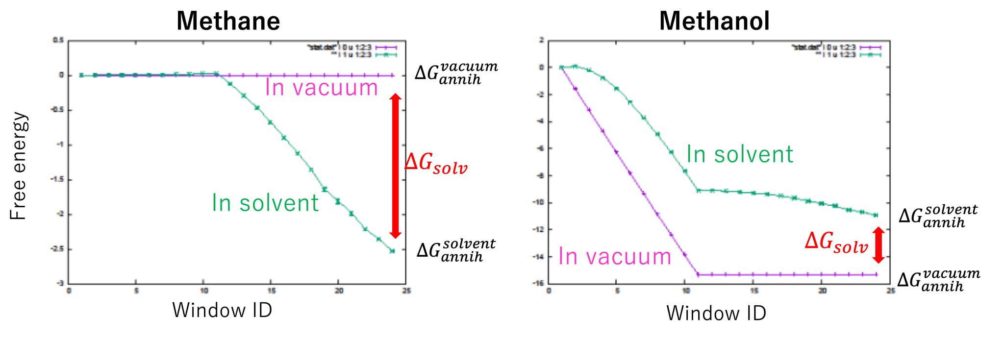
Figure 6. Free-energy changes from the initial state to the final state for “in solvent” and “in vacuum”.

Written by Hiraku Oshima@RIKEN BDR
March 31, 2022

References

Y. Sugita, A. Kitao, and Y. Okamoto, Multidimensional Replica-Exchange Method for Free-Energy Calculations. J. Chem. Phys. 113, 6042–6051 (2000). ↩
H. Fukunishi, O. Watanabe, S. Takada, On the Hamiltonian Replica Exchange Method for Efficient Sampling of Biomolecular Systems: Application to Protein Structure Prediction. J. Chem. Phys. 116, 9058−9067 (2002). ↩
M. Zacharias, T. P. Straatsma, and J. A. McCammon, Separation‐shifted scaling, a new scaling method for Lennard‐Jones interactions in thermodynamic integration. J. Chem. Phys. 100, 9025–9031 (1994). ↩
T. Steinbrecher, I. Joung, and D. A. Case, Soft-core potentials in thermodynamic integration: Comparing one- and two-step transformations. J. Comput. Chem. 32, 3253–3263 (2011). ↩
D. L. Mobley, J. P. Guthrie, FreeSolv: A Database of Experimental and Calculated Hydration Free Energies, with Input Files, J. Comput. Aided Mol. Des. 28, 711–720 (2014) ↩