GENESIS Tutorial 12.3 (2022)
gREST simulation of trialanine in water
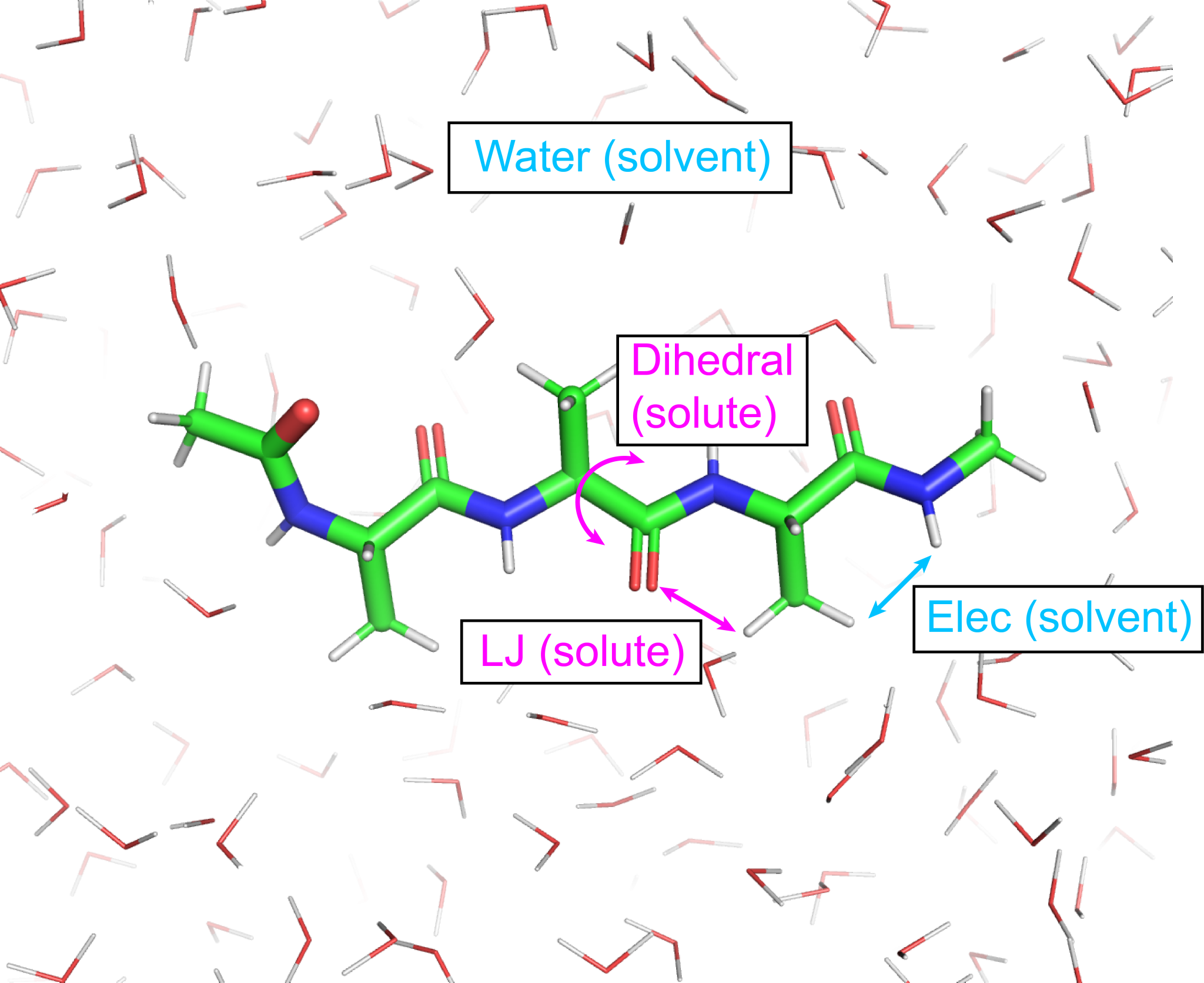
In this tutorial, we illustrate how to perform and analyze the replica exchange with solute tempering (REST) simulations for alanine tri-peptide. REST was originally developed by Berne et al.1, 2 to improve the performance of temperature replica exchange MD (T-REMD) simulations. Instead of increasing the temperature of the whole system, temperature of the “solute” region is virtually increased. This modification significantly reduces the required number of replicas. In GENESIS, new scheme of REST, referred to as generalized REST (gREST),3 is implemented. In gREST, the solute region is defined as a part of a molecule and/or a part of the potential energy terms. The rational choice of the solute region in the gREST framework effectively limits the energy space covered in REST and reduces the number of required replica. In the previous REMD tutorial, 20 replicas were needed while in this tutorial only 4 replicas are needed to cover the same temperature range.
When the temperature of the system (= target temperature) and the solute temperature are \(T_0\) and \(T_m\), respectively, the energy in gREST is modified as follows:
\[ \beta_0 U_{m} = \beta_0 \left[ \frac{\beta_m}{\beta_0} U_{\rm uu} + \left( \frac{\beta_m}{\beta_0}\right)^{l/n} U_{\rm uv} + U_{\rm vv} \right] , \]
where \(\beta_0\) and \(\beta_m\) are the inverse temperatures, \(u\) and \(v\) in the subscript represent the solute and solvent regions, respectively, and \(U_{uv}\) is the interaction between the solute and solvent. For example, the dihedral energy term can be used as the solute. Please note that in the temperature-REMD, each replica has the different temperature of the system, while in gREST all replicas have the same temperature of the system (= \(T_0\)). Only the potential energy (\(U_m\)) is changed by scaling the energy terms in the solute.
0. Preparations
All the files required for this tutorial are hosted in the GENESIS tutorials repository on GitHub. If you haven’t downloaded the files yet, open your terminal and run the following command (see more in Tutorial 1.1):
$ cd ~/GENESIS_Tutorials-2022
# if not yet
$ git clone https://github.com/genesis-release-r-ccs/genesis_tutorial_materials
If you already have the tutorial materials, let’s go to our working directory:
$ cd genesis_tutorial_materials/tutorial-12.3
1. Setup
To setup the system, please follow the steps in the basic tutorial (see Tutorial 3.2). We use the same input PDB and PSF files as in Tutorial 3.2.
# Prepare the input files
$ cd 1_setup
$ ln -s ../../tutorial-3.2/1_setup/3_solvate/wbox.pdb ./
$ ln -s ../../tutorial-3.2/1_setup/3_solvate/wbox.psf ./
2. Minimization and pre-equilibration
Non-physical steric clashes or non-equilibrium geometries in the initial
structure must be resolved before the gREST simulation. Here, we do this
via five steps:
1) minimization (step2.1),
2) equilibration in NVT ensemble (step2.2),
3) relaxation of the simulation box in NPT ensemble
with positional restraints (step2.3),
4) equilibration in NPT ensemble
without positional restraints (step 2.4),
5) equilibration in NPT ensemble with
3.5 fs time step and r-RESPA (step2.5).
In the 2_minimize_pre-equil directory, all control files step2.*.inp are
given. For further details of the control files and choice of parameters,
please refer to basic tutorials section (see Tutorial 3.2) and Tutorial 10.1
for simulations with large time step.
Let’s change directory.
#Change directory to 2_minimize_pre-equi
$ cd ../2_minimize_pre-equi
$ ls
step2.1.inp step2.2.inp step2.3.inp step2.4.inp step2.5.inp
2.1. Minimization
The first step of the simulation is to run energy minimization of the
system, in order to remove atomic clashes in the initial structure.
Please see following the important options in the control file step2.1.inp.
[INPUT]
topfile = ../toppar/top_all36_prot.rtf     # topology file
parfile = ../toppar/par_all36m_prot.prm    # parameter file
strfile = ../toppar/toppar_water_ions.str  # stream file
psffile = ../1_setup/wbox.psf              # protein structure file
pdbfile = ../1_setup/wbox.pdb              # PDB file

[OUTPUT]
dcdfile = step2.1.dcd          # DCD trajectory file
rstfile = step2.1.rst          # restart file

[ENERGY]
forcefield       = CHARMM  # [CHARMM]
electrostatic    = PME     # [PME]
switchdist       = 10.0    # switch distance
cutoffdist       = 12.0    # cutoff distance
pairlistdist     = 13.5    # pair-list distance
vdw_force_switch = YES     # force switch option for van der Waals
contact_check    = YES     # check atomic clash

[MINIMIZE]
method           = SD      # [SD]
nsteps           = 2000    # number of minimization steps
eneout_period    =   50    # energy output period
crdout_period    =   50    # coordinates output period
rstout_period    = 2000    # restart output period

[BOUNDARY]
type             = PBC     # [PBC]
box_size_x       = 50.2    # box size (x) in [PBC]
box_size_y       = 50.2    # box size (y) in [PBC]
box_size_z       = 50.2    # box size (z) in [PBC]

[SELECTION]
group1           = sid:PROA and heavy  # restraint group 1

[RESTRAINTS]
nfunctions       = 1        # number of functions
function1        = POSI     # restraint function type
direction1       = ALL      # direction [ALL,X,Y,Z]
constant1        = 1.0      # force constant
select_index1    = 1        # restrained groups
To execute the calculation, use the following command:
# Run energy minimization
$ export OMP_NUM_THREADS=5
$ mpirun -np 8 $GENESIS_BIN_DIR/spdyn step2.1.inp > step2.1.out
After the calculation, check the trajectory by using VMD. We can see that the atoms are slightly moved, but the atomic clashes are actually removed. In this step, we used 8 MPI processors and 5 OpenMP threads, namely, 40 CPU cores.
2.2. Equilibration of the system at 300 K
The second step of the simulation is to heat up the system, with
restraint on the peptide heavy atoms, to 300 K. The heating is performed
via annealing process wherein the temperature is increased by 3 K every
500 steps. Total simulation is 100 ps. Note that in this step the
integrator is Velocity Verlet (VVER) and Bussi thermostat.
Please see following the important options in
the control input file step2.2.inp.
[DYNAMICS]
integrator       =   VVER   # [LEAP,VVER]
nsteps           =  50000   # number of MD steps
timestep         =  0.002   # timestep (ps)
eneout_period    =    500   # energy output period
crdout_period    =    500   # coordinates output period
rstout_period    =  50000   # restart output period
annealing        =    YES   # simulated annealing
anneal_period    =    500   # annealing period
dtemperature     =      3   # temperature change at annealing (K)
iseed            =  31415   # random number seed

[CONSTRAINTS]
rigid_bond       = YES      # constraints all bonds involving hydrogen

[ENSEMBLE]
ensemble         = NVT      # [NVE,NVT,NPT,NPAT,NPgT]
tpcontrol        = BUSSI    # [NO,BERENDSEN,BUSSI,NHC]
temperature      = 0.1      # initial and target temperature (K)
To execute the simulation, we use similar commands as previous step.
# Run heating step
$ export OMP_NUM_THREADS=5
$ mpirun -np 8 $GENESIS_BIN_DIR/spdyn step2.2.inp > step2.2.out
2.3. Relaxation of the simulation box
After the system reached the desired temperature 300.00 K, we relax the
simulation box in NPT ensemble at 300 K and 1 atm for 50 ps.
Please see following the important options in the control file step2.3.inp.
[DYNAMICS]
integrator       =   VVER   # [LEAP,VVER]
nsteps           =  25000   # number of MD steps
timestep         =  0.002   # timestep (ps)
eneout_period    =    500   # energy output period
crdout_period    =    500   # coordinates output period
rstout_period    =  25000   # restart output period

[ENSEMBLE]
ensemble         = NPT      # [NVE,NVT,NPT,NPAT,NPgT]
tpcontrol        = BUSSI    # [NO,BERENDSEN,BUSSI,NHC]
temperature      = 300      # initial and target temperature (K)
pressure         = 1.0      # target pressure (atm)
To execute the simulation, we use the following command.
# Run relaxation of the system with restraints
$ export OMP_NUM_THREADS=5
$ mpirun -np 8 $GENESIS_BIN_DIR/spdyn step2.3.inp > step2.3.out
2.4. Equilibration with no positional restraints
We equilibrate all atom positions including the peptide atoms without
positional restraints (removes [RESTRAINTS]section). Here we turn on
the functions of hydrogen mass repartitioning (HMR) and group
temperature/pressure (group T/P) to use the 3.5 fs time step in the next
equilibration step. Please note that this option is only available in
GENESIS v2.0 and later.
Please see following the important options in the control file step2.4.inp.
[DYNAMICS]
integrator       =   VVER   # [LEAP,VVER,VRES]
nsteps           =  25000   # number of MD steps (50 ps)
timestep         =  0.002   # timestep (2 fs)
eneout_period    =    500   # energy output period
crdout_period    =    500   # coordinates output period
rstout_period    =  25000   # restart output period
hydrogen_mr      = yes      # Turn on HMR
hmr_ratio        = 3.0
hmr_ratio_xh1    = 2.0
hmr_target       = solute   # Apply HMR only to solute

[ENSEMBLE]
ensemble         = NPT      # [NVE,NVT,NPT,NPAT,NPgT]
tpcontrol        = BUSSI    # [NO,BERENDSEN,BUSSI,LANGEVIN]
temperature      = 300      # initial and target temperature (K)
pressure         = 1.0      # target pressure (atm)
group_tp         = YES      # usage of group tempeature and pressure
To run this step, we use the following command.
# Run equilbration without restraints
$ export OMP_NUM_THREADS=5
$ mpirun -np 8 $GENESIS_BIN_DIR/spdyn step2.4.inp > step2.4.out
2.5. Equilibration with 3.5 fs time step
Finally we run an additional 105 ps pre-equilibration simulation in NPT
ensemble. In this step, we equilibrate the system with the
multiple time step integrator, r-RESPA (VRES, timestep of 3.5 fs).
The integration with the longer time step requires HMR and group T/P options.
Please see following the important options in the control file step2.5.inp.
[DYNAMICS]
integrator        =   VRES  # [LEAP,VVER,VRES]
nsteps            =  30000  # number of MD steps (105 ps)
timestep          = 0.0035  # timestep (3.5 fs)
eneout_period     =    300  # energy output period (1.05 ps)
crdout_period     =    300  # coordinates output period (1.05 ps)
rstout_period     =  30000  # restart output period
nbupdate_period   =      6  # nonbond update period
elec_long_period  =      2  # period of reciprocal space calculation
thermostat_period =      6  # period of thermostat update
barostat_period   =      6  # period of barostat update
hydrogen_mr       = yes     # Turn on HMR
hmr_ratio         = 3.0
hmr_ratio_xh1     = 2.0
hmr_target        = solute  # Apply HMR only to solute

[ENSEMBLE]
ensemble         = NPT      # [NVE,NVT,NPT,NPAT,NPgT]
tpcontrol        = BUSSI    # [NO,BERENDSEN,BUSSI,LANGEVIN]
temperature      = 300      # initial and target temperature (K)
pressure         = 1.0      # target pressure (atm)
group_tp         = YES      # usage of group tempeature and pressure
To run this step, we use the following command.
# Run equilbration without restraints
$ export OMP_NUM_THREADS=5
$ mpirun -np 8 $GENESIS_BIN_DIR/spdyn step2.5.inp > step2.5.out
3. Equilibration for gREST
In this step, we equilibrate the system for each replica without replica exchange. Let’s move to the directory for equilibration of gREST.
#Change directory to 3_equilibrate
$ cd ../3_equilibrate
$ ls
step3.inp
The control file of gREST is very similar to that of T-REMD. The only
difference is that gREST needs select_indexN and param_typeN to
specify the “solute” region. The rest of system is regarded as “solvent”.
In this example, we define the the LJ and dihedral angle of
potential energy terms in Ala3 molecule as the solute region
(param_type1 = D L in [REMD] section and
group1 = ai:1-42 in [SELECTION] section).
In default, all of potential energy terms are treated as the solute
(param_type1 = ALL in [REMD] section).
If you want to treat other parts of potential energy terms as the solute,
param_typeN parameter may be modified (e.g. param_type1 = C CM to specify only charge and
CMAP terms as solute.).
We here use four replicas with the solute temperature range of 300.00 K
– 351.26 K (parameters1 = 300.00 318.12 337.14 351.26 in [REMD]
section) as a example. If you apply gREST to your system, you must
determine the number and the temperatures of replicas. To find the
number of replicas and temperatures, please refer to the appendix (see
Automatic Parameter Tuning for REMD, REUS, REST
). Each replica must be equilibrated at
the selected temperature just like conventional MD simulations. Note
that in this step as well as the next step (production run) we use NVT
ensemble. The r-RESPA integrator is combined with HMR and group T/P in
order to use 3.5 fs time step.
Please see following the important options in the control file step3.inp.
[REMD]
dimension        = 1            # number of parameter types
exchange_period  = 0            # NO exchange for equilibration
iseed            = 3141592
type1            = REST         # Replica Exchange with Solute Tempering
nreplica1        = 4            # number of replicas
parameters1      = 300.00 318.12 337.14 351.26 # list of solute temperatures
select_index1    = 1            # solute region selection
param_type1      = D L          # function types
                                # valid keywords are:
                                # ALL (default), BOND(B), ANGLE(A),
                                # DIHEDRAL(D), IMPROPER(I), CMAP(CM),
                                # CHARGE(C), LJ(L)...
                                # See manual for further details.

[SELECTION]
group1           = ai:1-42

[DYNAMICS]
integrator        =   VRES  # [LEAP,VVER,VRES]
nsteps            =  30000  # number of MD steps (105ps)
timestep          = 0.0035  # timestep (3.5fs)
eneout_period     =    300  # energy output period (1.05ps)
crdout_period     =    300  # coordinates output period (1.05ps)
rstout_period     =   3000  # restart output period
nbupdate_period   =      6  # nonbond update period
elec_long_period  =      2  # period of reciprocal space calculation
thermostat_period =      6  # period of thermostat update
barostat_period   =      6  # period of barostat update
hydrogen_mr       = yes     # Turn on HMR
hmr_ratio         = 3.0
hmr_ratio_xh1     = 2.0
hmr_target        = solute  # Apply HMR only to solute

[ENSEMBLE]
ensemble        = NVT       # [NVE,NVT,NPT]
tpcontrol       = BUSSI     # thermostat and barostat
temperature     = 300.0     # initial temperature (K)
pressure        = 1.0       # target pressure (atm)
group_tp        = YES
The following command performs a 105 ps NVT gREST simulations.
Here we use 160 (= 32 MPI x 5 OpenMP) CPU cores for the simulations.
# Run gREST equilibiration step
$ export OMP_NUM_THREADS=5
$ mpirun -np 32 $GENESIS_BIN_DIR/spdyn step3.inp > step3.out
4. Production
Since we have now completed all preparation steps, now we can start running the production simulation. Let’s move to the directory for production of gREST.
#Change directory
$ cd ../4_production
$ ls
step4.inp
We run a short simulation for 10.5 ns for the purpose of tutorial,
however longer simulation might be needed for conversion. The following
control file is used to run the simulation in NVT ensemble. One needs to
modify the control file for the equilibration such that
the exchange_period has a non-zero value (e.g. 3000 steps (10.5 ps))
and [INPUT] and [OUTPUT] files are properly refered. In order to
analyze the free energy, you need to select
the analysis_grest=YES in [REMD]. The option enables calculation of
energies with different solute temperatures. The energies with different
solute temperatures of each replica are written in step4_rep{}.ene.
Please see following the important options in the control file step4.inp:
[REMD]
dimension        = 1            # number of parameter types
exchange_period  = 3000         # exchange per 3000*3.5fs = 10.5 ps
type1            = REST         # Replica Exchange with Solute Tempering
nreplica1        = 4            # number of replicas
parameters1      = 300.00 318.12 337.14 351.26 # list of solute temperatures
select_index1    = 1            # solute region selection
param_type1      = D L          # function types
                                # valid keywords are:
                                # ALL (default), BOND, ANGLE,
                                # DIHEDRAL, IMPROPER, CMAP,
                                # CHARGE LJ...
                                # See manual for further details.
analysis_grest   = YES

[SELECTION]
group1           = ai:1-42

[DYNAMICS]
integrator        =    VRES # [LEAP,VVER,VRES]
nsteps            = 3000000 # number of MD steps (10.5 ns)
timestep          =  0.0035 # timestep (3.5 fs)
eneout_period     =     300 # energy output period (1.05 ps)
crdout_period     =     300 # coordinates output period (1.05 ps)
rstout_period     =   30000 # restart output period (105 ps)
nbupdate_period   =       6 # nonbond update period
elec_long_period  =       2 # period of reciprocal space calculation
thermostat_period =       6 # period of thermostat update
barostat_period   =       6 # period of barostat update
hydrogen_mr       = yes     # Turn on HMR
hmr_ratio         = 3.0
hmr_ratio_xh1     = 2.0
hmr_target        = solute  # Apply HMR only to solute

[ENSEMBLE]
ensemble         = NVT       # [NVE,NVT,NPT]
tpcontrol        = BUSSI     # thermostat and barostat
temperature      = 300.00    # K
group_tp         = YES       # usage of group tempeature and pressure
To run gREST production run, we use the following commands.
# Run gREST production step
$ export OMP_NUM_THREADS=5
$ mpirun -np 32 $GENESIS_BIN_DIR/spdyn step4.inp > step4.out
5. Analysis
In this tutorial, we mainly focus on calculating PMF of the end to end distance distribution at 300 K. In which, we use all temperatures trajectory upon applying the Multistate Bennett Acceptance Ratio (MBAR) re-weighting method.4 However, before calculating PMF, we first check the simulation by calculating acceptance ratio, replica random walk and temperature potential energy distribution.
In gREST control file, we setup the exchange_period=3000 which means
replica exchange is attempt every 10.5 ps. In the log output of the
gREST simulation, we can see the information about replica-exchange
attempts at every exchange_period steps.
REMD> Step:    2982000   Dimension:    1   ExchangePattern:    1
  Replica      ExchangeTrial             AcceptanceRatio      Before       After
        1          4 >     3   A         400 /       497     351.260     337.140
        2          2 >     1   A         394 /       497     318.120     300.000
        3          1 >     2   A         394 /       497     300.000     318.120
        4          3 >     4   A         400 /       497     337.140     351.260
  Parameter    :    337.140   300.000   318.120   351.260
  RepIDtoParmID:          3         1         2         4
  ParmIDtoRepID:          2         3         1         4
In this log file, we should pay attention to the AcceptanceRatio values. If those values are much lower than target, you should review the parameters of your simulation, such as modifying the temperature range. In this table, A and R indicate whether the exchange at this step is accepted or rejected, respectively. The last two columns show replica temperatures before and after the exchange trials, respectively.
The last three lines Parameter, RepIDtoParmID, and ParmIDtoRepID
summarize the locations and
parameters after replica exchanges. The Parameter line gives the
temperature of each replica in gREST simulation. The RepIDtoParmID
line stands for the permutation function that converts Replica ID to
Parameter ID. For example, in the 1st column, 3 is written, which
means that the temperature of Replica 1 is set to 337.140 K. The
ParmIDtoRepID line also represents the permutation function that
converts Parameter ID to Replica ID. For example, in the 3th column, 1
is written, which means that Parameter 3 (corresponding to the replica
temperature, 337.140 K) is located in Replica 1.
Now, please change the directory for analysis and proceed with the following steps:
# change directory
$ cd ../5_analysis
$ ls
1_calc_ratio  2_plot_index  3_sort  4_clac_dist  5_mbar  6_pmf
5.1. Calculate the acceptance ratio of each replica
Acceptance ratio of replica exchange is one of the important factors
that determine the efficiency of gREST simulations. The acceptance ratio
is displayed in a standard log output step4.out, and we examine the
data from the last step. Here, we show an example how to examine the
data. Note that the acceptance ratio of replica “A” to “B” is identical
to “B” to “A”, and thus we calculate only “A” to “B”. For this
calculation, you can use the script
calc_ratio.sh.
# change directory
$ cd 1_calc_ratio
$ ls
calc_ratio.sh

# make the file executable and use it
$ chmod u+x calc_ratio.sh
$ ./calc_ratio.sh

1 > 2 0.826
2 > 3 0.804
3 > 4 0.894
The file
calc_ratio.sh
contains the following commands:
# get acceptance ratios between adjacent parameter IDs
$ grep "  1 >     2" ../../4_production/step4.out | tail -1  > acceptance_ratio.dat
$ grep "  2 >     3" ../../4_production/step4.out | tail -1 >> acceptance_ratio.dat
$ grep "  3 >     4" ../../4_production/step4.out | tail -1 >> acceptance_ratio.dat

# calculate the ratios
$ awk '{print $2,$3,$4,$6/$8}' acceptance_ratio.dat
Note that the average acceptance ratio in this case is quite high, representing that a much larger temperature range can be achieved with fourreplicas. For consistency and comparison to REMD tutorial, the temperature range was kept the same.
5.2. Plot time courses of replica indices and temperatures
To examine the random walks of each replica in temperature space, we
analyze time course of the replica indices. We need to plot the values
of the ParmIDtoRepID lines from step4.out for a chosen starting
replica temperature, for example 300 K (first column), versus time.
Using following commands, we can get replica IDs in each snapshot.
# change directory
$ cd ../2_plot_index
$ ls
plot_index.sh plot_temperature.sh

# make the file executable and use it
$ chmod u+x plot_index.sh
$ ./plot_index.sh
The file
plot_index.sh
contains the following commands:
# get replica IDs in each snapshot
$ grep "ParmIDtoRepID:" ../../4_production/step4.out | sed 's/ParmIDtoRepID:/ /' > param.dat
Using following gnuplot commands, we can plot the replica IDs in each snapshot.
# make input file for gnuplot
cat << EOF > tmp.plt
set terminal png
set yrange [0:5]
set mxtics
set mytics
set xlabel "Time (ns)"
set ylabel "Replica ID"

# plot replica IDs which visited 300.00 K
set output "output_index1.png"
plot "param.dat" using (\$0*10.5/1000):1 with points pt 5 ps 0.5 lt 1 title "300.00 K"

# plot replica IDs which visited 318.12 K
set output "output_index2.png"
plot "param.dat" using (\$0*10.5/1000):2 with points pt 5 ps 0.5 lt 1 title "318.12 K"

# plot replica IDs which visited 337.14 K
set output "output_index3.png"
plot "param.dat" using (\$0*10.5/1000):3 with points pt 5 ps 0.5 lt 1 title "337.14 K"

# plot replica IDs which visited 351.26 K
set output "output_index4.png"
plot "param.dat" using (\$0*10.5/1000):4 with points pt 5 ps 0.5 lt 1 title "351.26 K"
EOF

# execute gnuplot
gnuplot ./tmp.plt
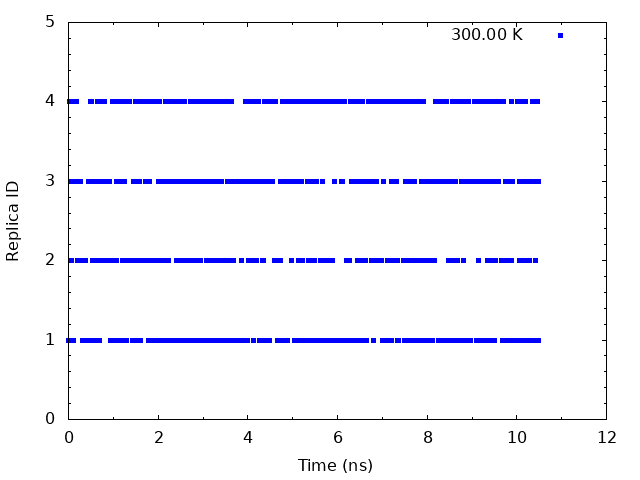
This graph indicate that the temperatures (300 K) visit randomly each replica, and thus random walks in the temperature spaces are successfully realized.
We also plot time courses of temperatures in one replica. We need to
plot one column in the Parameter : lines in step4.out versus time.
Using following commands. we can get replica temperatures in each
snapshot.
# make the file executable and use it
$ chmod u+x plot_temperature.sh
$ ./plot_temperature.sh
The file
plot_temperature.sh
contains the following commands:
# get replica temperatures in each snapshot
$ grep "Parameter    :" ../../4_production/step4.out | sed 's/Parameter    :/ /' > temperature.dat
As previous step, we can use gunplot script to plot the parameter IDs (= replica temperatures) in each snapshot.
# make input file for gnuplot
cat << EOF > tmp.plt
set term png
set mxtics
set mytics
set xlabel "Time (ps)"
set ylabel "Temperature (K)"
set output "output_temperature_rep1.png"
plot "temperature.dat" using (\$0*10.5/1000):1  with lines lc rgb "blue" title "repID=1 "
set output "output_temperature_rep2.png"
plot "temperature.dat" using (\$0*10.5/1000):2  with lines lc rgb "blue" title "repID=2 "
set output "output_temperature_rep3.png"
plot "temperature.dat" using (\$0*10.5/1000):3  with lines lc rgb "blue" title "repID=3 "
set output "output_temperature_rep4.png"
plot "temperature.dat" using (\$0*10.5/1000):4  with lines lc rgb "blue" title "repID=4 "
EOF

# execute gnuplot
gnuplot tmp.plt
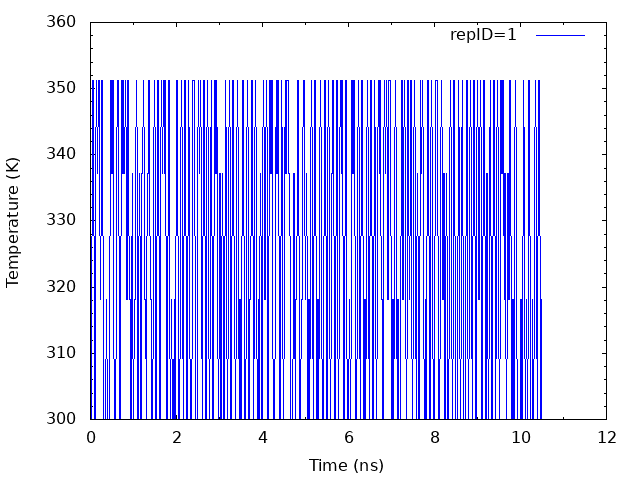
The temperatures of each replica during the simulation are distributed in all temperatures assigned. It means that correct annealing of the system is realized.
5.3. Sort coordinates in DCD trajectory files by parameters
The temperature in output DCD files of gREST simulation have all range
of temperatures, due to the exchange. Therefore, to analyze the
simulation further, we first need to sort the frames in the trajectory
based on their temperature. To do that, we use GENESIS analysis tool
remd_convert.
Sorting is done based on the information written in
remfiles generated from the gREST simulation.
Concomitantly, we also sort log and energy files
for each replica based on temperature parameters.
The sorted ene files will be used in the next step in MBAR analysis.
# change directory
$ cd ../3_sort
$ ls
remd_convert.inp

# Sort frames by parameters
$ $GENESIS_BIN_DIR/remd_convert remd_convert.inp | tee remd_convert.out
This example sorts the trajectory of the solute temperature of 300.00 K
(parameterID = 1) (convert_type = PARAMETER, convert_ids = 1 in [OPTION] section).
The system is aligned to the backbone of central alanine during the sorting
(fitting_atom = 2 in [FITTING] section, group2 = resno:2 and (an:N or an:CA or an:C or an:O) in [SELECTION] section),
and the water molecules are removed from the sorted trajectory (trjout_atom = 1 in [OPTION] section, group1 = ai:1-42 in [SELECTION] section).
The control file remd_convert.inp is as follows:
[INPUT]
psffile = ../../1_setup/wbox.psf
reffile = ../../1_setup/wbox.pdb
dcdfile = ../../4_production/step4_rep{}.dcd    # see remd_conv.sh
remfile = ../../4_production/step4_rep{}.rem    # see remd_conv.sh
enefile = ../../4_production/step4_rep{}.ene  # enefile of gREST

[OUTPUT]
pdbfile         = param.pdb    # pdbfile
trjfile         = param{}.dcd  # sorted dcdfile
enefile         = param{}.ene  # sorted enefile

[SELECTION]
group1          = ai:1-42   # only tri-alanine
group2          = resno:2 and (an:N or an:CA or an:C or an:O) # backbone of 2nd ALA

[FITTING]
fitting_method  = TR+ROT    # center-of-mass translation + rotation fitting
fitting_atom    = 2         # fitting to backbone of central alanine
mass_weight     = YES       # mass-weighted fitting

[OPTION]
check_only      = NO
convert_type    = PARAMETER
convert_ids     =           # 1 for only the lowest T replica; empty for all replicas
num_replicas    = 4
nsteps          = 3000000
exchange_period = 3000
crdout_period   = 300       # trjectory output frequency in REMD
eneout_period   = 300       # energy output frequency in REMD
trjout_format   = DCD
trjout_type     = COOR+BOX
trjout_atom     = 1         # output only tri-alanine moiety
pbc_correct     = NO        # nothing will happen when water mols excluded
Now we have sorted temperature log, ene and DCD file which will be used in the following analysis steps.
One can check the sorted trajectory by following commands:
# Check the sorted dcd file for ParameterID 1 (300.00 K)
$ vmd ./param.pdb ./param1.dcd
param*.ene files contain the energies at different solute
temperatures at the snapshots of each replica. For example, param1.ene
is shown below. The second column represents the potential energy at
300.00 K. The third, fourth, and fifth columns represent the potential
energies, which are estimated at 318.12 K, 337.14 K, and 351.26 K,
respectively, using the trajectory of 300.00
K.
 300       -38420.8021     -38420.7701     -38420.6700     -38420.5615
 600       -38437.8129     -38437.7333     -38437.5876     -38437.4485
 900       -38454.1105     -38454.6977     -38455.1828     -38455.4708
1200       -38523.4070     -38523.3613     -38523.2382     -38523.1079
1500       -38452.2631     -38452.5241     -38452.6885     -38452.7519
1800       -38472.7160     -38472.7599     -38472.7295     -38472.6667
5.4. Calculating end to end distance
In order to calculate the potential of the mean force (PMF) of the
end-to-end distance distribution, in the current subsection we calculate
the distance between the two terminal alanine OY_HNT.
# change directory
$ cd ../4_calc_distance
$ ls
calc_dist.sh

# make the file executable and execute the script
$ chmod u+x calc_dist.sh
$ ./calc_dist.sh
In the script calc_dist.sh, we use GENESIS analysis tool
trj_analysis as follows:
for i in 1 2 3 4; do

# Make input files for each Parameter ID.
cat << EOF > inp${i}
[INPUT]
reffile = ../3_sort/param.pdb

[OUTPUT]
disfile = param${i}.dis

[TRAJECTORY]
trjfile1      = ../3_sort/param${i}.dcd
md_step1      = 3000000         # number of MD steps
mdout_period1 = 300             # MD output period
ana_period1   = 300             # analysis period
repeat1       = 1
trj_format    = DCD             # (PDB/DCD)
trj_type      = COOR+BOX        # (COOR/COOR+BOX)
trj_natom     = 0               # (0:uses reference PDB atom count)

[OPTION]
check_only    = NO              # (YES/NO)
distance1     = PROA:1:ALA:OY PROA:3:ALA:HNT
EOF

# Execute trj_analysis
trj_analysis ./inp${i}

done
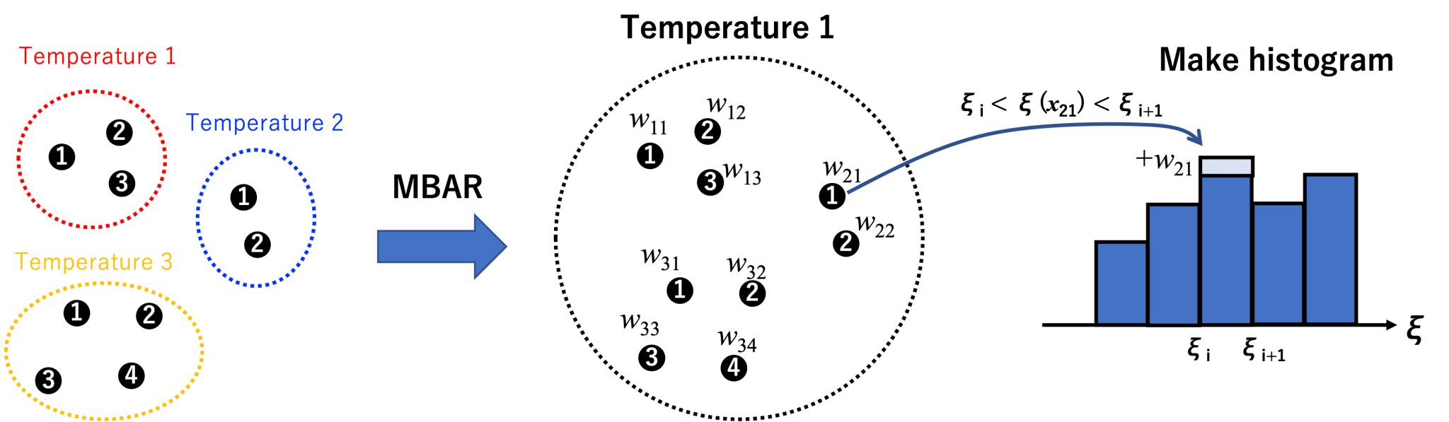
5.5. MBAR analysis
In order to use conformers from temperatures higher than the target temperature (300 K), we use the MBAR method. MBAR reweights each snapshot of each replica into the target temperature and provide the unbiased weight for each snapshot:
\[ W_{jn} = \frac{1}{c} \frac {\exp \left[-\beta_0U_0(x_{jn})\right]} {\sum_k N_k \exp \left[\beta_0 (f_k -U_k(x_{jn}))\right]}, \]
where \(x_{jn}\) is a configuration of snapshot \(n\) at replica
\(j\), \(f_k\) is the free energy of replica \(k\), and \(c\) is
a normalization constant. \(U_0\) is the potential energy function at
\(\beta_0\). \(U_k(x_{jn})\) corresponds to energies in
param*.ene files. Please note that the values of the solute
temperatures are not required for reweighting because their information
is already included in \(U_k(x_{jn})\).
We apply GENESIS mbar_analysis tool where we use our sorted energy
files as input cvfiles.
# change directory
$ cd ../5_mbar
$ ls
mbar_analysis.inp


# We run the analysis using the following command.
$ $GENESIS_BIN_DIR/mbar_analysis mbar_analysis.inp | tee mbar_analysis.log
The control file mbar_analysis.inp is as follows:
[INPUT]
cvfile             = ../3_sort/param{}.ene # input cv file

[OUTPUT]
fenefile           = fene.dat
weightfile         = weight{}.dat

[MBAR]
nreplica           = 4
input_type         = REST
dimension          = 1
nblocks            = 1
temperature        = 300.00
target_temperature = 300.00
input_type is set to REST to reweight gREST trajectories.
temperature and target_temperature are set to 300.00. As explained
above, the information about solute temperatures are not needed for
reweighting. mbar_analysis produces fene.dat file containing the
evaluated relative free energies and 4 “weight*.dat” files containing
the weights of each snapshot for each replica, which are reweighted to
300.00 K. For example, weight1.dat is shown below. The first line
corresponds to the weight of the first snapshot in param1.dcd. Each
weight represents the probability of each snapshot at 300.00 K.
$ head weight1.dat
         300  1.836119160862883E-005
         600  1.962571423551713E-005
         900  4.720421550879687E-006
        1200  1.883861114197157E-005
        1500  1.100339116123613E-005
        1800  1.636948804025372E-005
        2100  1.812549281313518E-005
        2400  2.113452205982935E-005
        2700  8.409791663698055E-006
        3000  1.536017798686323E-005
5.6. Calculating PMF of distance distribution
The final step of this tutorial is to use the calculated distances in
5.4. and weight files from MBAR analysis (5.5.) to calculate the PMF of
the end-to-end distance distribution in Ala3. We use another tool in
GENESIS pmf_analysis as follow:
# change directory
$ cd ../6_pmf
$ ls
pmf_analysis.inp plot_pmf.sh

# We run the analysis using the following command:
$ $GENESIS_BIN_DIR/pmf_analysis pmf_analysis.inp | tee pmf_analysis.log
The control file pmf_analysis.inp is as follows:
[INPUT]
cvfile       = ../4_calc_dist/param{}.dis
weightfile   = ../5_mbar/weight{}.dat

[OUTPUT]
pmffile      = dist.pmf

[OPTION]
nreplica     = 4             # number of replicas
dimension    = 1             # dimension of cv space
temperature  = 300.0
grids1       = 0 15 101      # (min max num_of_bins)
band_width1  = 0.1
is_periodic1 = NO            # periodicity of cv1
We plot the PMF using the provided script, plot_pmf.sh.
# make the file executable and plot PMF
$ chmod u+x plot_pmf.sh
$ ./plot_pmf.sh
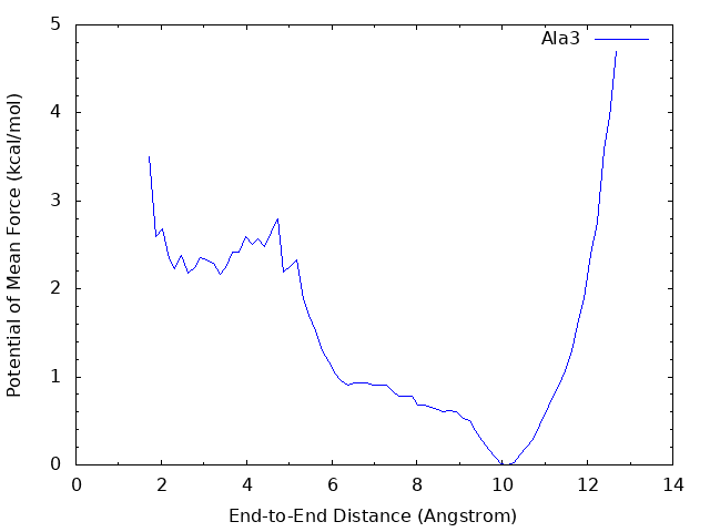
We can see that there is the global energy minimum around r = 10 Å and a local energy minimum around r = 2.8 Å. The latter corresponds to the α-helix conformation, where the hydrogen bond between OY and HNT is formed. These results suggest that in water the alanine tripeptide tends to form an extended conformation rather than α-helix.
Written Mar 1, 2018 by Motoshi Kamiya@RIKEN Computational biophysics
research team
Updated Feb 25, 2019 by Yasuhiro Matsunaga@RIKEN R-CCS
Updated Aug 31, 2019 by Suyong Re@RIKEN BDR
Updated Jul 2, 2020 by Chigusa Kobayashi@RIKEN R-CCS
Updated Jul 1, 2022 by Hisham Dokainish@RIKEN CPR
Updated Sep 14, 2022 by Hiraku Oshima@RIKEN BDR
References
-
P. Liu, B. Kim, R. A. Friesner, B. J. Berne, Proc. Natl. Acad. Sci. U.S.A.102, 13749–13754 (2005). ↩
-
L. Wang, R. A. Friesner, B. J. Berne, J. Phys. Chem. B 115, 9431–9438 (2011). ↩
-
M. Kamiya, Y. Sugita, J. Chem. Phys. 149, 072304 (2018). ↩
-
M. Shirts, J. D. Chodera, J. Chem. Phys., 129, 124105–124114 (2008). ↩