GENESIS Tutorial 12.2 (2022)
REUS for the (Ala)3 in water
Efficient conformational sampling is one of the difficult issues in the computational biophysics. Since complex biomolecules have many local-minimum energy states, conventional MD simulations often get trapped there. Umbrella sampling method has been widely used to calculate free energy profile. In 2000, Sugita et al. proposed the replica-exchange umbrella sampling method (REUS,1 which is also called Hamiltonian REMD2 or Window exchange umbrella sampling3), in which the restraint potentials are exchanged between replicas to enhance conformational sampling. In this tutorial, we demonstrate a REUS simulation of a small peptide using GENESIS.
0. Preparation
All the files required for this tutorial are hosted in the GENESIS tutorials repository on GitHub.
If you haven’t downloaded the files yet, open your terminal and run the following command (see more in Tutorial 1.1):
$ cd ~/GENESIS_Tutorials-2022
# if not yet
$ git clone https://github.com/genesis-release-r-ccs/genesis_tutorial_materials
If you already have the tutorial materials, let’s go to our working directory:
# Let's take a note
$ echo "tutorial-12.2: REUS simulation for ala3" >> README

# Check out the contents in Tutorial 12.2
$ cd genesis_tutorial_materials/tutorial-12.2
Since we use the CHARMM force field, we make a symbolic link to the CHARMM toppar directory (see Tutorial 2.2).
# Make a symbolic link to the CHARMM toppar directory
$ ln -s ../../Data/Parameters/toppar_c36_jul21 ./toppar
$ ln -s ../../Programs/genesis-2.0/bin ./
$ ls
1_setup              3_equilibrate  5_analysis  toppar
2_minimize_pre-equi  4_production   bin
This tutorial consists of five steps: 1) system setup, 2) energy minimization and pre-equilibration, 3) equilibration, 4) production run, and 5) trajectory analysis. Control files for GENESIS are already included in the file.
1. Setup
In this tutorial, we simulate the (Ala)3 in water. We use the same input PDB and PSF files as in Tutorial 3.2.
# Prepare the input files
$ cd 1_setup
$ ln -s ../../tutorial-3.2/1_setup/3_solvate/wbox.pdb ./
$ ln -s ../../tutorial-3.2/1_setup/3_solvate/wbox.psf ./
2. Minimization and pre-equilibration
Similar to the conventional MD simulations, we carry out an energy minimization for the initial structure, followed by a short MD simulation to equilibrate the system. We use the same protocols described in Tutorial 3.2. Since we have already equilibrated the system in Tutorial 3.2, we use the restart file obtained previously.
# Take over the restart file obtained in Tutorial 3.2
$ cd ../2_minimize_pre-equi
$ ln -s ../../tutorial-3.2/3_equilibrate/eq3.rst
3. Equilibration
Final goal of this tutorial is to calculate the free energy profile (or potential of mean force) as a function of the end-to-end distance of the (Ala)3. We are going to use 14 replicas in the REUS simulation. Since each replica has an individual restraint potential, we have to equilibrate the system using 14 different restraints before the production run. Let’s take a look at the control file:
# change directory
$ cd ../3_equilibrate
# check the control file (only important sections are shown below)
$ less INP
[INPUT]
topfile = ../toppar/top_all36_prot.rtf # topology file
parfile = ../toppar/par_all36m_prot.prm # parameter file
strfile = ../toppar/toppar_water_ions.str # stream file
psffile = ../1_setup/wbox.psf # protein structure file
pdbfile = ../1_setup/wbox.pdb # PDB file
rstfile = ../2_minimize_pre-equi/eq3.rst # restart file
[OUTPUT]
logfile = eq_rep{}.log # log file of each replica
dcdfile = eq_rep{}.dcd # DCD trajectory file
remfile = eq_rep{}.rem # parameter index file
rstfile = eq_rep{}.rst # restart file
[REMD]
dimension = 1
exchange_period = 0
type1 = RESTRAINT
nreplica1 = 14
cyclic_params1 = NO
rest_function1 = 1
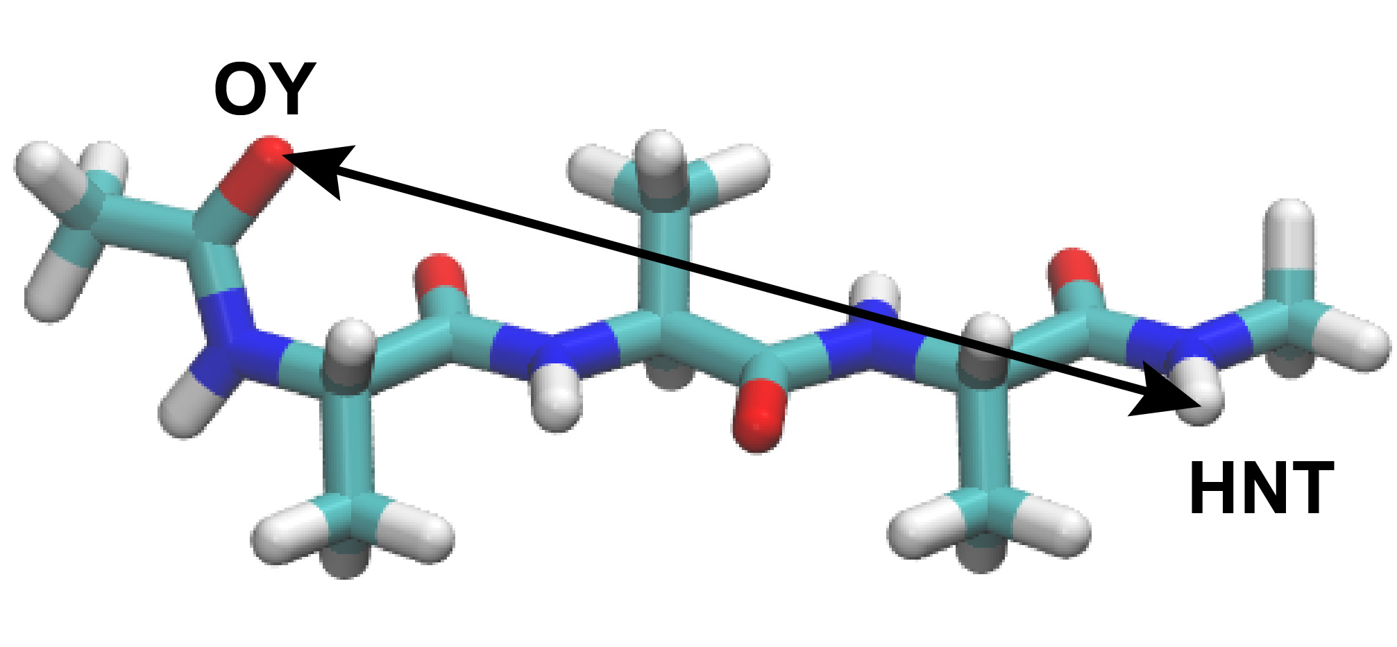
[SELECTION]
group1 = an:OY and resno:1 # restraint group 1
group2 = an:HNT and resno:3 # restraint group 2
[RESTRAINTS]
nfunctions = 1
function1 = DIST
constant1 = 1.2 1.2 1.2 1.2 1.2 1.2 1.2 1.2 1.2 1.2 1.2 1.2 1.2 1.2
reference1 = 1.80 2.72 3.64 4.56 5.48 6.40 7.32 8.24 9.16 10.08 11.00 11.92 12.84 13.76
select_index1 = 1 2
This control file is almost same with the subsequent production run of
the REUS simulation. Here, we specify exchange_period = 0 in
the [REMD] section, which means that parameter exchange is not
attempted during the simulation. In the [REMD], [SELECTION], and
[RESTRAINTS] sections, we give REUS parameters. We apply restraints on
the distance between the OY atom in Residue 1 and HNT atom in Residue 3.
The target distance is ranging from 1.80 to 13.76 Å at the interval of
0.92 Å, and the force constant of the restraint potential is set to 1.2
kcal/mol/Å2 for all replicas. Note that 1.80 Å is nearly corresponding
to the hydrogen bond distance, and 13.76 Å is a distance when the
peptide forms a fully extended conformation.
Index of the restraint function used in REUS is specified in [REMD] section by rest_function,
and the restraint function is further defined in [RESTRANTS] section.
Note that, in the [REMD] section, the suffix on rest_function (e.g. the “1” in rest_function1)
denotes the REMD dimension and must match the suffix on other [REMD] settings such as
type, nreplica, and cyclic_params;
the value assigned to rest_function (the number after the =) is the restraint index.
In the [RESTRAINTS] section, that same restraint index must serve as the suffix on
function, constant, reference, and select_index to define the corresponding parameters.
Note that the values in the same column of the constant and reference lines
are packed into one “parameter set” to be set to and exchanged between replicas.
Specifically, if the user sets
constant1 = 1.2 1.4 1.6 and reference1 = 1.80 2.72 3.64,
replicas receive the sets (1.2, 1.80), (1.4, 2.72) or (1.6, 3.64).
In the [OUTPUT] section, we can see that there is a bracket {} in
the filename. The replica number is automatically inserted into this
bracket. For example, Replica1 yields eq_rep1.log, eq_rep1.dcd,
and eq_rep1.rst. As for the other sections, we use common parameters
to the conventional MD simulations (see Tutorial 3.2). The
simulation is performed in the NVT ensemble at 300 K, and Bussi
thermostat is used for the temperature control. The SHAKE/RATTLE and
SETTLE algorithms are applied to the bonds including hydrogen and TIP3P
water, respectively. We carry out 200 ps MD simulation for each replica.
If you are going to employ the NVT ensemble in the production run, you should NOT use the NPT ensemble at this stage. Otherwise, each replica has different volume in the production run.
Now, let’s execute spdyn. Since we have 14 replicas, the total number
of MPI processors should be 14 × n, where n is the number of MPI
processors employed for each replica. If you specify multiple OpenMP
threads with “export OMP_NUM_THREADS=m”, the total number of CPU cores
used for the simulation should be 14 × n × m. Please, specify the
correct number of processors in your batch script, when you run the
simulation. The following is an example command, in which 32 CPU cores
are employed for one replica (448 CPU cores in total).
# Carry out the equilibration run
$ mpirun -np 112 -x OMP_NUM_THREADS=4 ../bin/spdyn INP > log
Number of MPI processors in each replica is automatically set to “total MPI processors ÷ number of replicas”. In addition, each replica keeps the rule of hybrid MPI/OpenMP parallelization for single MD simulation.
Let’s check the peptide conformation in the trajectory of each replica by using VMD. We can see that the conformation in Replica 1 (short distance restraint) is compact, while it is extended in Replica 14 (long distance restraint), indicating that the equilibration runs with 14 individual restrains were correctly done.
# for Replica 1
$ vmd ../1_setup/wbox.pdb -psf ../1_setup/wbox.psf -dcd eq_rep1.dcd

# for Replica 14
$ vmd ../1_setup/wbox.pdb -psf ../1_setup/wbox.psf -dcd eq_rep14.dcd
4. Production run
We carry out a production run of the REUS simulation. Let us see the control file. The following shows important options.
# Change directory for production run
$ cd ../4_production

# View the control file
$ less INP
[INPUT]
topfile = ../1_setup/top_all36_prot.rtf     # topology file
parfile = ../1_setup/par_all36m_prot.prm    # parameter file
strfile = ../1_setup/toppar_water_ions.str  # stream file
psffile = ../1_setup/wbox.psf               # protein structure file
pdbfile = ../1_setup/wbox.pdb               # PDB file
rstfile = ../3_equilibrate/eq_rep{}.rst     # restart file

[OUTPUT]
logfile = prod_rep{}.log     # log file of each replica
dcdfile = prod_rep{}.dcd     # DCD trajectory file
rstfile = prod_rep{}.rst     # restart file
remfile = prod_rep{}.rem     # parameter index file

[REMD]
dimension         = 1
exchange_period   = 2000
type1             = RESTRAINT
nreplica1         = 14
cyclic_params1    = NO
rest_function1    = 1

[DYNAMICS]
integrator        = VRES     # RESPA integrator
nsteps            = 4000000  # MD steps in one replica
timestep          = 0.0025   # timestep (ps)
eneout_period     = 200      # energy output period
crdout_period     = 200      # coordinates output period
rstout_period     = 4000000  # restart output period
nbupdate_period   = 10       # nonbond update period
elec_long_period  = 2        # period of reciprocal space calculation
thermostat_period = 10       # period of thermostat update
barostat_period   = 10       # period of barostat update
The main difference from the previous pre-equilibration run is
exchange_period = 2000 in the [REMD] section. The parameter
exchange is attempted every 2,000 steps. In the [OUTPUT] section, we
define remfile, where the parameter index in each replica is output
during the simulation. We perform 10-ns REUS simulation for each replica
(10 ns × 14 replicas = 140 ns in total). Coordinates are output every
200 steps. Like the previous equilibration run, we execute spdyn.
# Perform production run
$ mpirun -np 112 -x OMP_NUM_THREADS=4 ../bin/spdyn INP > log
In the log file, information about replica-exchange attempt is output at
every exchange_period step. For example, at 154,000 step you can see the
following information (detailed results might be different from yours):
REMD> Step: 154000   Dimension: 1   ExchangePattern: 2
  Replica   ExchangeTrial    AcceptanceRatio   Before   After
        1        1 >    0  N        0 /    0        1       1
        2        2 >    3  R        7 /   39        2       2
        3        8 >    9  R        6 /   39        8       8
        4        3 >    2  R        7 /   39        3       3
        5        4 >    5  R       12 /   39        4       4
        6        6 >    7  R       10 /   39        6       6
        7        7 >    6  R       10 /   39        7       7
        8        5 >    4  R       12 /   39        5       5
        9       11 >   10  R       11 /   39       11      11
        10      14 >    0  N        0 /    0       14      14
        11      13 >   12  A       18 /   39       13      12
        12      12 >   13  A       18 /   39       12      13
        13       9 >    8  R        6 /   39        9       9
        14      10 >   11  R       11 /   39       10      10

Parameter    :   1   2   8   3   4   6   7   5  11  14  12  13   9  10
RepIDtoParmID:   1   2   8   3   4   6   7   5  11  14  12  13   9  10
ParmIDtoRepID:   1   2   4   5   8   6   7   3  13  14   9  11  12  10
In this case,
Replica 11 had Parameter 13 (k = 1.2, r = 12.84) before 154,000 step,
and the exchange to Parameter 12 (k = 1.2, r = 11.92) was accepted (A) at 154,000 step,
and then it has Parameter 12 after 154,000 step.
The acceptance ratio between the parameter pairs 12 and 13 at 154,000 step is 18/39 (=46.2%).
Replica 5 had Parameter 4 (k = 1.2, r = 4.56),
but the exchange to Parameter 5 (k = 1.2, r = 5.48) was rejected (R), and
then it has still Parameter 4 after 154,000 step.
Replicas 1 and 10 have Parameters 1 and 14, respectively, but
they have no neighboring pairs. Thus, replica exchange was not attempted (N) at this step.
We can see that ExchangePattern is 2 at 154,000 step
(end of the first line).
In the case of ExchangePattern = 2, Parameters 2-3, Parameters 4-5, Parameters 6-7,
…, and Parameters 12-13 are defined as the neighboring pairs.
On the other hand, in the case of ExchangePattern = 1, Parameters 1-2, Parameters 3-4,
Parameters 5-6, …, and Parameters 13-14 are defined as the neighboring pairs.
In the one-dimensional REMD simulation, ExchangePattern = 1 and 2
emerge alternatively at every exchange_period.
The last three lines Parameter, RepIDtoParmID, and ParmIDtoRepID
summarize location of replica and parameter indexes.
The RepIDtoParmID stands for the permutation function that converts Replica
ID to Parameter ID. For example, in the 3rd column, 8 is written, which
means that Replica 3 has Parameter 8. In the 9th column, 11 is written,
indicating that Replica 9 has Parameter 11.
The ParmIDtoRepID also stands for the permutation function that converts Parameter ID to
Replica ID. For example, in the 3rd column, 4 is written, which means
that Parameter 3 is located in Replica 4. In the 5th column, 8 is
written, indicating that Parameter 5 is located in Replica 8.
The Parameter line includes parameter index of each replica. In the case of
REUS, this line is same with RepIDtoParmID line.
After the simulation is finished, we obtain trajectory and restart files from each replica.
If you want to restart the REUS simulation, do NOT change the order of the replica parameters in the control file before and after the restart, even if parameter exchange occurred during the simulation.
[RESTRAINTS]
constant1  =  1.2  1.2  1.2  1.2  1.2  1.2  1.2  1.2  1.2   1.2   1.2   1.2   1.2   1.2
reference1 = 1.80 2.72 3.64 4.56 5.48 6.40 7.32 8.24 9.16 10.08 11.00 11.92 12.84 13.76
5. Analysis
In this section, we explain how to analyze REUS trajectories. All
analyses are carried out in the 5_analysis directory.
# change directory
$ cd ../5_analysis
$ ls
1_convert_dcd  2_sort_dcd  3_calc_ratio  4_plot_index  5_calc_dist  6_calc_mbar  7_calc_pmf
5.1. Make converted trajectory files for analysis
Since the obtained “raw” DCD files contain many water molecules, it may
take much time to analyze them. In order to save time, we first remove
all water molecules from the trajectory files, and create new DCD files
by using crd_convert. In addition, we superimpose the peptide
structure of each snapshot onto the initial structure. Sample control
file for crd_convert is already prepared in the 1_dcd_convert
directory. For this purpose, we need 14 control files in total. These
files were created with a script in the script directory.
# Change directory
$ cd 1_convert_dcd
$ ls
INP1   INP11  INP13  INP2  INP4  INP6  INP8  run.csh
INP10  INP12  INP14  INP3  INP5  INP7  INP9  script

# Run crd_convert for each
$ ../../bin/crd_convert INP1 > log1
$ ../../bin/crd_convert INP2 > log2
:
$ ../../bin/crd_convert INP14 > log14

# check the converted trajectory file by VMD
$ vmd replica1.pdb -dcd replica1.dcd
5.2. Sort coordinates in DCD files by parameters
In the raw DCD files generated from the REUS simulation, coordinates at
different conditions (or replica parameters) are mixed. In order to sort
the coordinates by replica parameters, we use remd_convert. Sorting is
done based on the information in the remfile. In the 2_sort_dcd
directory, sample control file is already prepared.
# Change directory
$ cd ../2_sort_dcd

# View the control file
$ less INP
[INPUT]
reffile = ../1_convert_dcd/replica1.pdb      # PDB file
dcdfile = ../1_convert_dcd/replica{}.dcd     # DCD file
remfile = ../../4_production/prod_rep{}.rem  # REMD parameter ID file
logfile = ../../4_production/prod_rep{}.log  # REMD energy log file

[OUTPUT]
pdbfile = param.pdb             # PDB file
trjfile = param{}.dcd           # trajectory file
logfile = param{}.log           # REMD energy log file

[SELECTION]
group1          = all           # selection group 1

[FITTING]
fitting_method  = NO            # method

[OPTION]
convert_type    = PARAMETER     # (REPLICA/PARAMETER)
convert_ids     =               # selected index (empty = all)
num_replicas    = 14            # total number of replicas
nsteps          = 4000000       # nsteps in [DYNAMICS]
exchange_period =    2000       # exchange_period in [REMD]
crdout_period   =     200       # crdout_period in [DYNAMICS]
eneout_period   =     200       # eneout_period in [DYNAMICS]
trjout_format   = DCD           # (PDB/DCD)
trjout_type     = COOR+BOX      # (COOR/COOR+BOX)
trjout_atom     = 1             # atom group
centering       = NO            # shift center of mass
pbc_correct     = NO            # (NO/MOLECULE)
In the [INPUT] section, we specify dcdfile and PDB file obtained in
the previous subsection. This is because input dcdfile should contain
the same number and order of atoms with reffile. Of course, you can
specify the original DCD and PDB files
(../../4_production/step4_rep{}.dcd and ../../1_setup/wbox.pdb) for
dcdfile and reffile, but it takes a very long time for trajectory
convert, because they contain many water molecules. In the [OPTION]
section, convert_type = PARAMETER is used to sort coordinates by
replica parameters. Here, nsteps, exchange_period, crdout_period,
and eneout_period must be idential to those used in the REUS
simulation. We run remd_convert by the following command, and then
obtain the sorted trajectory files.
# Run remd_convert
$ ../../bin/remd_convert INP > log

# Check the sorted dcd file for Parameter 1 (r = 1.80)
$ vmd param.pdb -dcd param1.dcd
5.3. Calculate the acceptance ratio
Acceptance ratio of the parameter exchange is one of the important factors that determine an efficiency of REMD simulations. The acceptance ratio is displayed in the log file as mentioned above, and we examine the data at the last step. Here, we show an example command to collect and summarize the data. Note that the acceptance ratio of “A to B” is identical to “B to A”, and we calculate only “A to B”. The averaged acceptance ratio was ~0.25, indicating that sufficient replica exchange was realized in the simulation.
# Change directory
$ cd ../3_calc_ratio

# Get the acceptance ratio between neighboring parameter pairs
$ grep ' 1 >     2' ../../4_production/log | tail -1 >  log
$ grep ' 2 >     3' ../../4_production/log | tail -1 >> log
$ grep ' 3 >     4' ../../4_production/log | tail -1 >> log
:
$ grep '13 >    14' ../../4_production/log | tail -1 >> log

# Show the results
$ awk '{print $2,$3,$4,$6/$8}' log
1 > 2 0.343
2 > 3 0.22
3 > 4 0.116
4 > 5 0.162
5 > 6 0.269
6 > 7 0.225
7 > 8 0.178
8 > 9 0.172
9 > 10 0.261
10 > 11 0.267
11 > 12 0.268
12 > 13 0.326
13 > 14 0.427
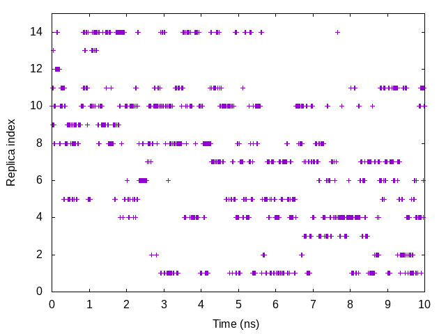
5.4. Plot the time courses of replica index and target distance
To examine a random walk of the system in replica space, we analyze the
time courses of the replica index. We need to plot one column in the
ParmIDtoRepID: lines in log onto the time axis. The following
commands are example to plot the replica index that has Parameter 10 (k = 1.2 kcal/mol/Å2 and r = 10.08Å):
# Change directory
$ cd ../4_plot_index

# Create log file that contains replica index
$ grep "ParmIDtoRepID:" ../../4_production/log > index.log

# Plot the time courses of replica index that has Parameter 10
$ gnuplot
gnuplot> set xlabel 'Time (ns)'
gnuplot> set ylabel 'Replica index'
gnuplot> unset key
gnuplot> plot [][0:15]'index.log' u ($0/200):11
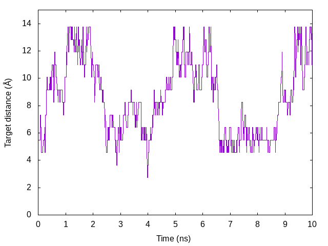
We also plot the time courses of the target distance of the restraint
function in one replica. In the log file, parameter index is output in
the Parameter : lines instead of the target distance. So, we should
convert the index to the actual distance value. Here, we use awk script
(./script/convert.awk) to convert them. The following commands are
example to plot the target distance in Replica 5.
# Create log file that contains target distance
$ grep "Parameter    :" ../../4_production/log > param.log
$ awk -f ./script/convert.awk param.log > dist.log

# Plot the time courses of target distance in Replica 5
$ gnuplot
gnuplot> set xlabel 'Time (ns)'
gnuplot> set ylabel 'Target distance (Å)'
gnuplot> unset key
gnuplot> plot [][0:15]'dist.log' u ($0/200):5 with lines
5.5. Analyze the end-to-end distance of (Ala)3
In this subsection, we calculate the end-to-end distance of the (Ala)3
by using trj_analysis. In the 5_calc_dist directory, we have two
directories: replica and parameter. The former is used to analyze
the original DCD files (../1_convert_dcd/replica{}.dcd), and the
latter is used to analyze the sorted DCD files
(../2_sort_dcd/param{}.dcd).
# Change directory
$ cd ../5_calc_dist
$ ls
parameter  replica
First, let us calculate the end-to-end distance of the peptide in the original DCD file. Sample control files are already contained in the directory. Again, we have to prepare 14 individual control files to analyze each replica.
# Change directory
$ cd replica
$ ls
INP1   INP11  INP13  INP2  INP4  INP6  INP8  run.csh
INP10  INP12  INP14  INP3  INP5  INP7  INP9  script

# Check one control file
$ less INP1
[INPUT]
reffile = ../../1_convert_dcd/replica1.pdb        # PDB file

[OUTPUT]
disfile = replica1.dis                            # distance file

[TRAJECTORY]
trjfile1      = ../../1_convert_dcd/replica1.dcd  # trajectory file
md_step1      = 4000000                       # number of MD steps
mdout_period1 = 200                           # MD output period
ana_period1   = 200                           # analysis period
repeat1       = 1
trj_format    = DCD                           # (PDB/DCD)
trj_type      = COOR+BOX                      # (COOR/COOR+BOX)
trj_natom     = 0                             # (0:uses reference PDB atom count)

[OPTION]
check_only    = NO
distance1     = PROA:1:ALA:OY PROA:3:ALA:HNT
INP1 is used to analyze ../../1_convert_dcd/replica1.dcd. Because
the DCD file should contain the same number and order of atoms with the
input PDB file, we specify ../../1_convert_dcd/replica1.pdb as
reffile. Here, we compute the distance between OY atom in Ala1 and HNT
atom in Ala3. After running trj_analysis for INP1 to INP14, we
obtain replica1.dis to replica14.dis. We plot the time courses of
the distance in Replica 5 below as an example.
# Run trj_analysis to analyze the distance
# this is done for 1 to 14 (./run.csh is available for scripting)
$ ../../../bin/trj_analysis INP1 > log1
$ ../../../bin/trj_analysis INP2 > log2
:
$ ../../../bin/trj_analysis INP14 > log14

# Plot the time courses of the distance in Replica 5
$ gnuplot
gnuplot> set xlabel 'Time (ns)'
gnuplot> set ylabel 'Distance (Å)'
gnuplot> unset key
gnuplot> plot [][0:15]'replica5.dis' u ($0/2000):2 with lines
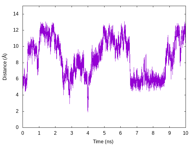
Let us compare the results with the above plot (changes in the target distance in Replica 5). We can see that the distance increases as the target distance increases, and vice versa.
Then, let us calculate the end-to-end distance in the sorted DCD
files. Sample control files are already contained in the
./5_calc_dist/parameter directory. Again, we should prepare 14
individual control files to analyze each DCD file. After
running trj_analysis, we obtain parameter1.dis to parameter14.dis
as the output files. We plot the histogram of the end-to-end distance
obtained in each restraint condition by using gnuplot. There are 20,000
distance data in each file, and we set the bin width to be 0.05Å.
# Change directory
$ cd ../parameter
$ ls
INP1   INP11  INP13  INP2  INP4  INP6  INP8  run.csh
INP10  INP12  INP14  INP3  INP5  INP7  INP9  script

# Run trj_analysis to analyze the distance
$ ../../../bin/trj_analysis INP1 > log1
$ ../../../bin/trj_analysis INP2 > log2
:
$ ../../../bin/trj_analysis INP14 > log14

# Plot the histogram of the end-to-end distance
$ gnuplot
gnuplot> set key outside
gnuplot> set xlabel 'Distance (Å)'
gnuplot> set ylabel 'Probability'
gnuplot> binwidth=0.05
gnuplot> bin(x,width)=width*floor(x/width)
gnuplot> ndata=20000
gnuplot> plot for [k=1:14] 'parameter'.k.'.dis' u (bin($2,binwidth)):(1.0/ndata) w l t 'Parameter'.k smooth freq
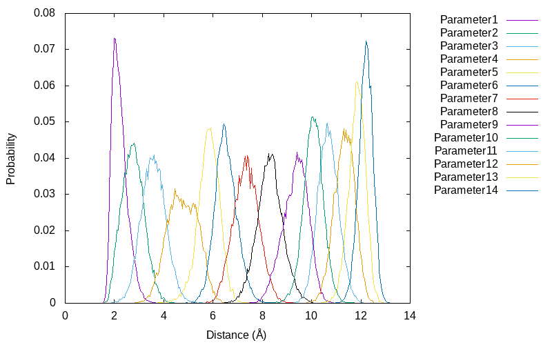
The results show that there is enough overlap between neighboring umbrella windows along the reaction coordinates. These overlaps are important to obtain reliable free energy profile in reweighting techniques such as WHAM.
5.6. Free energy calculation using MBAR
We calculate the free energy profile of the (Ala)3 as a function of
the end-to-end distance by using MBAR. Here, we use mbar_analysis of
the GENESIS analysis tool set. Let us move to the 6_calc_mbar
directory, and see the sample control file:
# change directory
$ cd ../../6_calc_mbar
$ less INP
[INPUT]
cvfile = ../5_calc_dist/parameter/parameter{}.dis # Collective variable file

[OUTPUT]
fenefile   = output.fene      # free energy file
weightfile = output{}.weight  # weight file

[MBAR]
nreplica           = 14
input_type         = CV
dimension          = 1
nblocks            = 1
temperature        = 300
target_temperature = 300
rest_function1     = 1

[RESTRAINTS]
constant1      = 1.2 1.2 1.2 1.2 1.2 1.2 1.2 1.2 1.2 1.2 1.2 1.2 1.2 1.2
reference1     = 1.80  2.72  3.64  4.56  5.48  6.40  7.32  \
                 8.24  9.16 10.08 11.00 11.92 12.84 13.76
is_periodic1   = NO
In the [INPUT] section, we specify the output file generated from the
distance analysis for the sorted DCD files (see the previous subsection). In the [MBAR] section, we set the number of the dimension
of the reaction coordinates, the temperature used in the REUS
simulation, and so on. For the [RESTRAINTS] section, we give the same
information used in the REUS control file.
# perform mbar
$ ../../bin/mbar_analysis INP > log
This produces output.fene file containing the evaluated relative
free energies and 14 output*.weight files containing the weights of
each snapshot for each replica. For example, output1.weight is as
follows:
$ less output1.weight
           1   1.4097966267636603E-007
           2   1.5805208264591707E-007
           3   1.5488288652400664E-007
           4   1.4596171898407404E-007
           5   1.6880812728502563E-007
           6   1.8985319931591140E-007
           7   1.4525835770429576E-007
           :
           :
       19997   1.4189940392490833E-007
       19998   1.6620382169517072E-007
       19999   1.4418046201344524E-007
       20000   1.5028161473380590E-007
5.7. Calculating PMF of distance distribution
The final step of this tutorial is to use the calculated distances in
5.5 and weight files from MBAR analysis (5.6) to calculate PMF of end to
end distance distribution in (Ala)3. Here, we use pmf_analysis of
the GENESIS analysis tool set. Let us move to the 7_calc_pmf
directory, and see the sample control file:
# change directory
$ cd ../7_calc_pmf
$ less INP

[INPUT]
cvfile      = ../5_calc_dist/parameter/parameter{}.dis # collective variable file
weightfile  = ../6_calc_mbar/output{}.weight           # weight file

[OUTPUT]
pmffile     = dist.pmf        # potential of mean force file

[OPTION]
nreplica     = 14            # number of replicas
dimension    = 1             # dimension of cv space
temperature  = 300
grids1       = 0.0 15.0 601  # (min max num_of_bins)
band_width1  = 0.25  # sigma of gaussian kernel
                     # should be comparable or smaller than the grid size
                     # (pmf_analysis creates histogram by accumulating gaussians)
is_periodic1 = NO    # periodicity of cv1

# perform pmf
$ ../../bin/pmf_analysis INP > log

# plot the PMF of end to end distance
$ gnuplot
gnuplot> set xlabel 'Distance (Å)'
gnuplot> set ylabel 'Potential of mean force (kcal/mol)'
gnuplot> plot [0:13][0:10]'dist.pmf' u 1:3 w lines
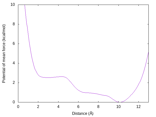
We can see that there is the global energy minimum around r = 10.1 Å and a local energy minimum around r = 2.8 Å. The latter corresponds to the α-helix conformation, where the hydrogen bond between OY and HNT is formed. These results suggest that in water the (Ala)3 tends to form an extended conformation rather than α-helix. Note that this 10-ns simulation might be still short to get a reliable free energy profile. The users are strongly recommended to check the convergence of the free energy profile. If you extend the simulation time, and the free energy profile was largely changed, your simulation might be still short (or structure sampling is not sufficient).4
Written by Takaharu Mori@RIKEN Theoretical molecular science laboratory
Created April 26, 2022
Updated by Haeri Im @ RIKEN Theoretical molecular science laboratory
July 28, 2022