GENESIS Tutorial 12.1 (2022)

REMD simulation of (Ala)₃ in water

In this tutorial, we illustrate how to run temperature replica exchange molecular dynamics (T-REMD) simulations of (Ala)₃ and calculate PMF of end to end distance and dihedral angle (Φ and Ψ) distribution. T-REMD is an enhanced sampling method that parallelly simulate the system at a range of different temperatures and periodically exchanging between them. As a result of sampling at several temperature, the simulation can efficiently overcome well known problem of conventional MD, wherein the conformation could be trapped in a local minimum. For further details of REMD method, please refer to the original paper.¹

REMD simulation in GENESIS requires an MPI environment. At least one MPI processor must be assigned to one replica.

Please note that it may take more than 12 hours to finish all simulations in this tutorial.

python 3.x.x is required for analysis in this tutorial.

Preparation

All the files required for this tutorial are hosted in the GENESIS tutorials repository on GitHub. If you haven’t downloaded the files yet, open your terminal and run the following command (see more in Tutorial 1.1):

$ cd ~/GENESIS_Tutorials-2022
# if not yet
$ git clone https://github.com/genesis-release-r-ccs/genesis_tutorial_materials

If you already have the tutorial materials, let’s go to our working directory:

$ cd genesis_tutorial_materials/tutorial-12.1

This tutorial consists of five steps: 1) system setup, 2) energy minimization and pre-equilibration, 3) REMD equilibration, 4) REMD production, and 5) trajectory analysis. Control files for GENESIS are already included in the download file. Since we use the CHARMM36m force field parameters,² we make a symbolic link to the CHARMM toppar directory (see Tutorial 2.2).

$ ln -s ../../Data/Parameters/toppar_c36_jul21 ./toppar
$ ls 
1_setup  2_min_equil  3_equil_remd  4_prod_remd  5_analy toppar

1. Setup

In this tutorial, we simulate (Ala)₃ in explicit water. We use the same initial structure as in Tutorial 3.2.

# Change directory for the system setup
$ cd 1_setup 

# Prepare PDB and PSF files
$ ln -s ../../tutorial-3.2/1_setup/3_solvate/wbox.pdb ./
$ ln -s ../../tutorial-3.2/1_setup/3_solvate/wbox.psf ./

2. Minimization and pre-equilibration

We use the same protocols described in Tutorial 3.2. Since we have already equilibrated the system in Tutorial 3.2, we use the restart file obtained previously.

# Change directory for the minimization and equilibration
$ cd ../2_minimize_pre-equi

# Prepare equilibrated restart file
$ ln -s ../../tutorial-3.2/3_equilibrate/eq3.rst

3. REMD equilibration

Temperature setting

Before starting T-REMD simulation, we must determine the number of replicas and the temperatures of replicas. These temperatures need to be chosen carefully, because they will greatly affect the results of T-REMD simulations and probabilities of the replica exchanges. If the difference of temperatures between adjacent replicas is small, the exchange probability is high, but the number of replicas needed for such simulation is also large. Therefore, we need to find the optimal temperature intervals to perform efficient REMD simulations.

We recommend using the web server REMD Temperature generator.³ This tool automatically generates the number of replicas and their temperatures according to the information we input. We show the example of the input for the T-REMD simulation of the solvated trialanine system:

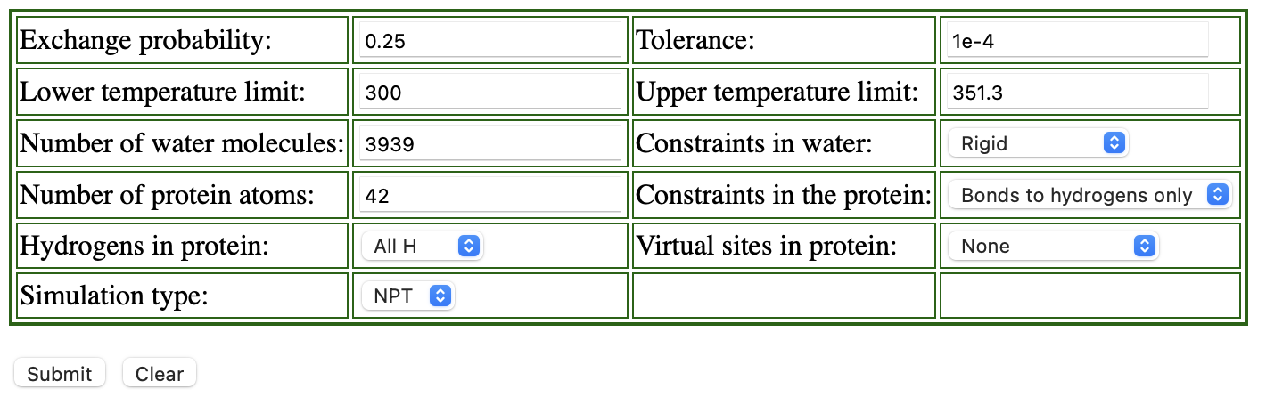
Replica exchange probabilities are often set to 0.2 – 0.3, and here we set the replica exchange probability to 0.25. The lower and upper temperature limits are set to 300 K and 351.3 K, respectively. Since we use SHAKE and SETTLE algorithms in the simulation, “constraints in the protein” is set to “Bonds to hydrogen only”, and “Constraints in water” to “rigid”. We use all-atom model, so we select “All H” for the parameter of “Hydrogens in proteins”. The numbers of protein atoms and the water molecules are input according to the numbers in ../1_setup/wbox.pdb. We can count the number of the water molecules in the system as follows:

# Count the number of TIP3P water molecules
$ grep "TIP3" ../1_setup/wbox.pdb | wc -l | awk '{print $1 / 3}'

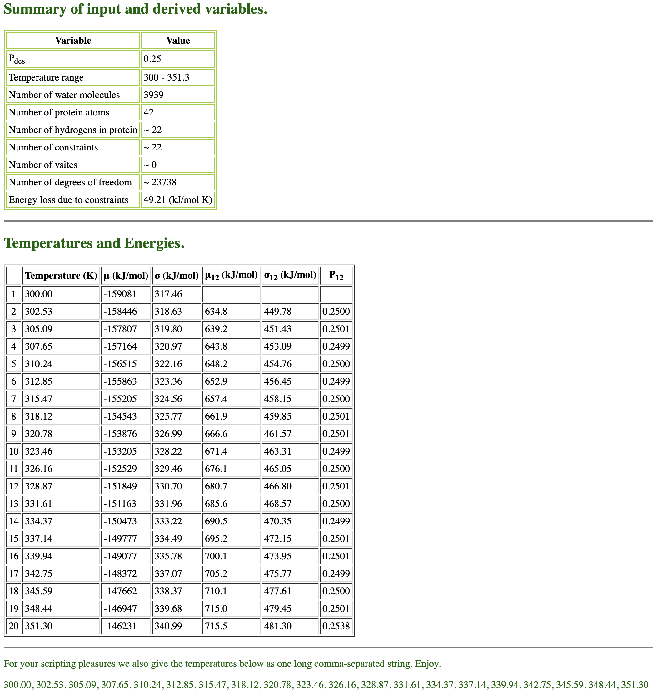
When we fill in all the parameters and submit them, the server generates the summary, temperatures and energies of 20 replicas in a few seconds as follows.
In the table shown above, there is the parameter “Simulation type”. We can select either “NPT” or “NVT” for the parameter, but, when we select “NVT”, the server returns an error message. Thus we choose “NPT” here, even though we use NVT ensemble in our T-REMD simulation.

Equilibration

# Change directory for the REMD equilibration
$ cd ../3_equil_remd
$ ls
run.inp

Using generated temperature parameters, we start our REMD simulation. First, each replica must be equilibrated at the selected temperature just like conventional MD simulations. The following command performs a 500 ps NVT MD simulations with run.inp. This equation of motion are integrated with the RESPA integrator (VRES) with the time step of 2.5 fs, where the SHAKE algorithm is used for bond constraint. Make sure that you use NVT ensemble, as using NPT ensemble make significant differences in the potential energy of each replica and subsequently hinder the exchange between them. The REMD equilibration control file is:

[INPUT]
topfile  = ../toppar/top_all36_prot.rtf     # topology file
parfile  = ../toppar/par_all36m_prot.prm    # parameter file
strfile  = ../toppar/toppar_water_ions.str  # stream file
psffile  = ../1_setup/wbox.psf              # protein structure file
pdbfile  = ../1_setup/wbox.pdb              # PDB file
reffile  = ../1_setup/wbox.pdb              # PDB file
rstfile  = ../2_min_equil/eq3.rst          # restart file

[OUTPUT]
dcdfile  = run_rep{}.dcd         # DCD trajectory file
rstfile  = run_rep{}.rst         # restart file
remfile  = run_rep{}.rem         # replica exchange ID file
logfile  = run_rep{}.log         # log file of each replica

[ENERGY]
forcefield        = CHARMM       # CHARMM force field
electrostatic     = PME          # use Particle mesh Ewald method
switchdist        = 10.0         # switch distance
cutoffdist        = 12.0         # cutoff distance
pairlistdist      = 13.5         # pair-list distance
pme_nspline       = 4            # order of the spline interpolation
vdw_force_switch  = YES          # turn on vdw force switch
pme_max_spacing   = 1.2          # Max grid spacing allowed
    
[DYNAMICS]
integrator        = VRES         # [LEAP,VVER,VRES]
nsteps            = 200000       # number of MD steps
timestep          = 0.0025       # timestep (ps)
eneout_period     = 2000         # energy output period
crdout_period     = 2000         # coordinates output period
rstout_period     = 20000        # restart output period
nbupdate_period   = 10           # pairlist update period
elec_long_period  = 2            # period of reciprocal space calculation
thermostat_period = 10           # period of thermostat update
barostat_period   = 10           # period of barostat update

[CONSTRAINTS]
rigid_bond        = YES          # use SHAKE/RATTLE
fast_water        = YES          # use SETTLE

[ENSEMBLE]
ensemble          = NVT          # [NVE,NVT,NPT]
tpcontrol         = BUSSI        # thermostat and barostat
temperature       = 300          # K
group_tp          = YES          # group temperature/pressure evaluation

[BOUNDARY]
type              = PBC          # periodic boundary condition

[REMD]
dimension         = 1            # number of parameter types
exchange_period   = 0            # NO exchange for equilibration
type1             = TEMPERATURE  # T-REMD
nreplica1         = 20           # number of replicas
parameters1       = 300.00 302.53 305.09 307.65 310.24 \
                    312.85 315.47 318.12 320.78 323.46 \
                    326.16 328.87 331.61 334.37 337.14 \
                    339.94 342.75 345.59 348.44 351.30

In [INPUT] section, we specify ../2_min_equil/eq3.rst file as the restart file of the simulation run. In the REMD simulation, the 20 (equal to the number of replicas specified nreplica in [REMD] section explained below) copies are automatically made from this restart file.

In [OUTPUT] section, in addition to dcdfile and rstfile names, we give also logfile and remfile. If we perform REMD simulations, file names of logfile and remfile are also required. logfile gives a log file of MD simulation for each replica. The remfile gives replica exchange parameter. In this section, “{}” returns a replica index number from 1 to 20.

When we want to run REMD simulations, we add [REMD] section in the control file. In [REMD] section, the number of dimensions is set to dimension = 1, and the type of the exchanged variable is set to type1 = temperature for T-REMD simulation. The number of replicas is set to nreplica1 = 20, and we assign the replica temperatures to the variable parameter1. If exchange_period = 0, then no exchanges occur during the run, and so we set exchange_period to 0 for equilibration of all replicas.

In [ENSEMBLE] section, we use NVT ensemble in this tutorial. Though we can perform REMD simulations both in NVT and NPT ensemble with GENESIS, we recommend performing T-REMD simulations in NVT ensemble, because in a temperature exceeding the water boiling point, the system may be disrupted.

To run REMD equilibiration, we use the following commands. Here we used 8 MPI processes and 4 OpenMP threads for each replica, i.e., a total of 640 (= 8 x 4 x 20) CPU cores.

# Run REMD-equilibiration step. 
$ export OMP_NUM_THREADS=4
$ mpirun -np 160 /home/user/GENESIS/bin/spdyn run.inp > run.log

4. REMD production

# Change directory for the REMD production
$ cd ../4_prod_remd
$ ls
run.inp

Since we have now completed all preparation steps, now we can start running the production simulation. We ran a short simulation for 10 ns for the purpose of tutorial, however longer simulation is actually needed to obtain better energy results. The following control file is used to run the simulation in NVT ensemble:

[INPUT]
topfile  = ../toppar/top_all36_prot.rtf     # topology file
parfile  = ../toppar/par_all36m_prot.prm    # parameter file
strfile  = ../toppar/toppar_water_ions.str  # stream file 
psffile  = ../1_setup/wbox.psf              # protein structure file
pdbfile  = ../1_setup/wbox.pdb              # PDB file
reffile  = ../1_setup/wbox.pdb              # PDB file
rstfile  = ../3_equil_remd/run_rep{}.rst    # restart file

[OUTPUT]
dcdfile  = run_rep{}.dcd         # DCD trajectory file
rstfile  = run_rep{}.rst         # restart file
remfile  = run_rep{}.rem         # replica exchange ID file
logfile  = run_rep{}.log         # log file of each replica

[ENERGY]
forcefield        = CHARMM       # CHARMM force field
electrostatic     = PME          # use Particle mesh Ewald method
switchdist        = 10.0         # switch distance
cutoffdist        = 12.0         # cutoff distance
pairlistdist      = 13.5         # pair-list distance
pme_nspline       = 4            # order of the spline interpolation
vdw_force_switch  = YES          # turn on vdw force switch
pme_max_spacing   = 1.2          # Max grid spacing allowed

[DYNAMICS]
integrator        = VRES         # [LEAP,VVER,VRES]
nsteps            = 4000000      # number of MD steps
timestep          = 0.0025       # timestep (ps)
eneout_period     = 2000         # energy output period
crdout_period     = 2000         # coordinates output period
rstout_period     = 20000        # restart output period
nbupdate_period   = 10           # pairlist update period
elec_long_period  = 2            # period of reciprocal space calculation
thermostat_period = 10           # period of thermostat update
barostat_period   = 10           # period of barostat update

[CONSTRAINTS]
rigid_bond        = YES          # use SHAKE/RATTLE
fast_water        = YES          # use SETTLE
  
[ENSEMBLE]
ensemble          = NVT          # [NVE,NVT,NPT]
tpcontrol         = BUSSI        # thermostat and barostat
pressure          = 1            # atm
temperature       = 300          # K
group_tp          = YES          # group temperature/pressure evaluation

[BOUNDARY]
type              = PBC          # periodic boundary condition

[REMD]
dimension         = 1            # number of parameter types
exchange_period   = 2000         # NO exchange for equilibration
type1             = TEMPERATURE  # T-REMD
nreplica1         = 20           # number of replicas
parameters1       = 300.00 302.53 305.09 307.65 310.24 \
                    312.85 315.47 318.12 320.78 323.46 \
                    326.16 328.87 331.61 334.37 337.14 \
                    339.94 342.75 345.59 348.44 351.30

In [INPUT] section, rstfile points to the output files from the equilibration. “{}” returns a series of the 20 input files.

In [REMD] section, the period between replica exchanges is specified by exchange_period = 2000. Then replica exchange attempts occurs every 2000 steps, that is, every 5 (=2000 x 0.025) ps.

The other parameters in [REMD] section should not be changed from those in the input files of your previous runs.

To run REMD production, we use the following commands. Here we used 8 MPI processes and 4 OpenMP threads for each replica, i.e., a total of 640 (= 8 x 4 x 20) CPU cores.

# Run REMD production 
$ export OMP_NUM_THREADS=4
$ mpirun -np 160 /home/user/GENESIS/bin/spdyn run.inp > run.log

5. Analysis

In this tutorial, we mainly focus on calculating PMF of the end to end distance and dihedral angle distribution at 300 K. In which, we use all temperatures trajectory upon applying the Multistate Bennett Acceptance Ratio (MBAR) re-weighting method. For information on MBAR method, please refer to the original paper.⁴

End to end distance of (Ala)₃

Dihedral angle of (Ala)₃

In REMD control file, we setup the exchange_period=2000. In the log output of the REMD simulation, we can see the information about replica-exchange attempts at every exchange_period steps.

REMD> Step:    1998000   Dimension:    1   ExchangePattern:    2
  Replica      ExchangeTrial             AcceptanceRatio      Before       After
        1          3 >     2   R         148 /       500     305.090     305.090
        2          6 >     7   A         171 /       500     312.850     315.470
        3          1 >     0   N           0 /         0     300.000     300.000
        4          4 >     5   R         170 /       500     307.650     307.650
        5         11 >    10   R         199 /       500     326.160     326.160
        6          7 >     6   A         171 /       500     315.470     312.850
        7          8 >     9   R         178 /       500     318.120     318.120
        8         17 >    16   A         198 /       500     342.750     339.940
        9          2 >     3   R         148 /       500     302.530     302.530
       10         20 >     0   N           0 /         0     351.300     351.300
       11         18 >    19   A         200 /       500     345.590     348.440
       12         13 >    12   R         208 /       500     331.610     331.610
       13         10 >    11   R         199 /       500     323.460     323.460
       14          9 >     8   R         178 /       500     320.780     320.780
       15          5 >     4   R         170 /       500     310.240     310.240
       16         12 >    13   R         208 /       500     328.870     328.870
       17         15 >    14   R         184 /       500     337.140     337.140
       18         16 >    17   A         198 /       500     339.940     342.750
       19         14 >    15   R         184 /       500     334.370     334.370
       20         19 >    18   A         200 /       500     348.440     345.590

  Parameter    :    305.090   315.470   300.000   307.650   326.160   312.850   318.120   339.940   302.530   351.300   348.440   331.610   323.460   320.780   310.240   328.870   337.140   342.750   334.370   345.590
  RepIDtoParmID:          3         7         1         4        11         6         8        16         2        20        19        13        10         9         5        12        15        17        14        18
  ParmIDtoRepID:          3         9         1         4        15         6         2         7        14        13         5        16        12        19        17         8        18        20        11        10

REMD> Step:    2000000   Dimension:    1   ExchangePattern:    1
  Replica      ExchangeTrial             AcceptanceRatio      Before       After
        1          3 >     4   A         183 /       500     305.090     307.650
        2          7 >     8   R         173 /       500     315.470     315.470
        3          1 >     2   R         240 /       500     300.000     300.000
        4          4 >     3   A         183 /       500     307.650     305.090
        5         11 >    12   R         152 /       500     326.160     326.160
        6          6 >     5   A         167 /       500     312.850     310.240
        7          8 >     7   R         173 /       500     318.120     318.120
        8         16 >    15   A         174 /       500     339.940     337.140
        9          2 >     1   R         240 /       500     302.530     302.530
       10         20 >    19   A         229 /       500     351.300     348.440
       11         19 >    20   A         229 /       500     348.440     351.300
       12         13 >    14   A         177 /       500     331.610     334.370
       13         10 >     9   R         153 /       500     323.460     323.460
       14          9 >    10   R         153 /       500     320.780     320.780
       15          5 >     6   A         167 /       500     310.240     312.850
       16         12 >    11   R         152 /       500     328.870     328.870
       17         15 >    16   A         174 /       500     337.140     339.940
       18         17 >    18   R         177 /       500     342.750     342.750
       19         14 >    13   A         177 /       500     334.370     331.610
       20         18 >    17   R         177 /       500     345.590     345.590

  Parameter    :    307.650   315.470   300.000   305.090   326.160   310.240   318.120   337.140   302.530   348.440   351.300   334.370   323.460   320.780   312.850   328.870   339.940   342.750   331.610   345.590
  RepIDtoParmID:          4         7         1         3        11         5         8        15         2        19        20        14        10         9         6        12        16        17        13        18
  ParmIDtoRepID:          3         9         4         1         6        15         2         7        14        13         5        16        19        12         8        17        18        20        10        11

In this log file, we should pay attention to the AcceptanceRatio values. In this table, 'A' and 'R' mean that the exchange at this step is accepted or rejected respectively. The last two columns show replica temperatures before and after the exchange trials respectively.

The Parameter, RepIDtoParmID, and ParmIDtoRepID lines summarize the locations and parameters after replica exchanges. The Parameter line gives the temperature of each replica in T-REMD simulation. The RepIDtoParmID line stands for the permutation function that converts Replica ID to Parameter ID. For example, in the 1st column, 4 is written, which means that the temperature of Replica 1 is set to 307.65 K. The ParmIDtoRepID line also represents the permutation function that converts Parameter ID to Replica ID. For example, in the 5th column, 6 is written, which means that Parameter 5 (corresponding to the replica temperature, 310.24 K) is located in Replica 6.

In REMD preparation step using temperature generator, we setup the probability of exchange to 0.25. So we first check the simulation acceptance ratio and check if it matches our original selection, see next section.

# change directory 
$ cd ../5_analy
$ ls 
1_calc_ratio  3_sort            5_end_end_distance  7_MBAR         9_PMF_dihedral
2_plot_index  4_plot_potential  6_dihedral_angle    8_PMF_distance

5.1. Calculate the acceptance ratio of each replica

As we mentioned in the previous section, acceptance ratio of replica exchange is one of the important factors that determine the efficiency of REMD simulations. The acceptance ratio is displayed in a standard log output “../4_prod_remd/run.log”, and we examine the data from the last step. Here, we show an example how to examine the data. Note that the acceptance ratio of replica “A” to “B” is identical to “B” to “A”, and thus we calculate only “A” to “B”. For this calculation, you can use the script “calc_ratio.sh”.

# change directory 
$ cd 1_calc_ratio 

# make the file executable and use it 
$ chmod u+x calc_ratio.sh 
$ ./calc_ratio.sh 

 1 >  2 0.399 
 3 >  4 0.401 
 5 >  6 0.379 
 7 >  8 0.369 
 9 > 10 0.415 
11 > 12 0.393 
13 > 14 0.414 
15 > 16 0.425 
17 > 18 0.434 
19 > 20 0.413 

The file “calc_ratio.sh” contains the following commands:

# get acceptance ratios between adjacent parameter IDs
$ grep "  1 >     2" ../../4_prod_remd/run.log | tail -1  > acceptance_ratio.dat
...
...
$ grep " 19 >    20" ../../4_prod_remd/run.log | tail -1 >> acceptance_ratio.dat

# calculate the ratios
awk '{printf ("%2d %s %2d %4.3f \n", $2,$3,$4,$6/$8)}' acceptance_ratio.dat

5.2. Plot time courses of replica indices and temperatures

To examine the random walks of each replica in temperature space, we analyze “time course of the replica indices for each set temperature” and “time courses of temperatures in one replica”. First, we analyze time course of the replica indices for each set temperature. We need to plot the values of the “ParmIDtoRepID” lines from ../4_prod_remd/run.log for a chosen starting replica temperature versus time. Each column correspond to initial set temperature respectively. For example, the first column correspond to 300 K, the 10th column correspond to 323.46 K, and the last column correspond to 351.3 K. Using following commands, we can get replica IDs in each snapshot.

# change directory
$ cd ../2_plot_index 
$ ls
$ plot_index.sh plot_temperature.sh plot_repID-Tempreture.gnuplot plot_parmID-repID.gnuplot 

# make the file executable and use it
$ chmod u+x plot_index.sh
$ ./plot_index.sh

# plot replica IDs in each snapshot 
$ gnuplot plot_parmID-repID.gnuplot

The file “plot_index.sh” contains the following commands:

# get replica IDs in each snapshot
grep "ParmIDtoRepID:" ../../4_prod_remd/run.log | sed 's/ParmIDtoRepID:/ /' > T-REMD_parmID-repID.dat

The file “plot_parID-repID.gnuplot” contains the following commands :

set terminal jpeg
reset
set yrange [0:22]set mxtics
set mytics
set xlabel "Time (ns)"
set ylabel "Replica ID"

set output "300.00k.jpg"
plot "T-REMD_parmID-repID.log" using ($1*0.0025*0.001):2  with points pt 5 ps 0.5 lt 1 title "300.00 K"

set output "323.46k.jpg"
plot "T-REMD_parmID-repID.log" using ($1*0.0025*0.001):11 with points pt 7 ps 0.5 lt 2 title "323.46 K"

set output "351.30k.jpg"
plot "T-REMD_parmID-repID.log" using ($1*0.0025*0.001):21 with points pt 9 ps 0.5 lt 3 title "351.30 K"

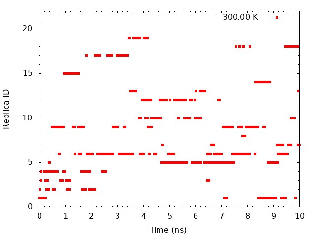
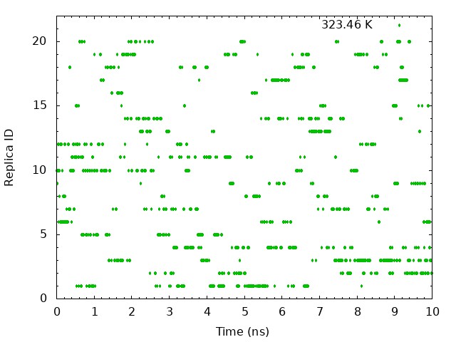
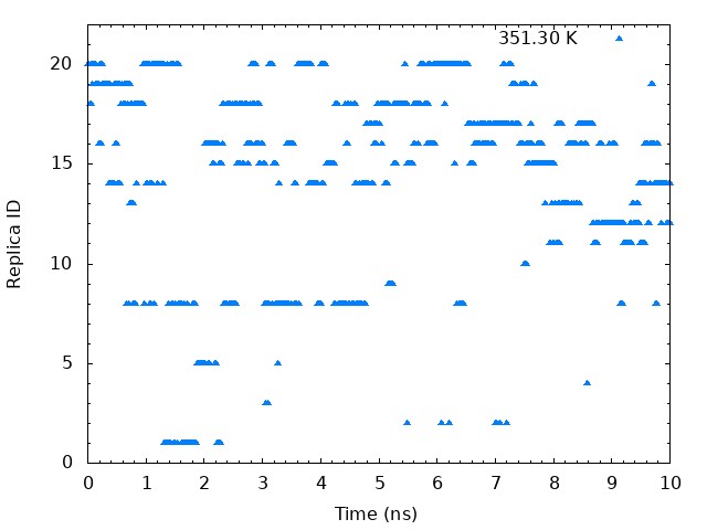
These graphs indicate that a certain temperature (parameterID) visit randomly each replica, and thus random walks in the temperature spaces are realized.

Next, we plot time courses of temperatures in one replica. We need to plot one column in the “Parameter :” lines in ../4_prod_remd/run.log versus time. Using following commands. we can get replica temperatures in each snapshot.

# make the file executable and use it
$ chmod u+x plot_temperature.sh
$ ./plot_temperature.sh

# plot tempreture IDs in each snapshot 
$ gnuplot plot_repID-Temperature.gnuplot

The file “plot_temperature.sh” contains the following commands:

# get replica temperatures in each snapshot
grep "Parameter    :" ../../4_prod_remd/run.log | sed 's/Parameter    :/ /' > T-REMD_repID-temperatrue.dat

The “plot_repID-Temperature.gnuplot” include the following commands:

set terminal jpeg
set output "RepID1_10_20.jpg"
set yrange [300:360]set mxtics
set mytics
set xlabel "Time (ns)"
set ylabel "Temperature (K)"
plot \
  "T-REMD_repID-Temperature.log" using ($1*0.0025*0.001):2  with lines lt 3 title "repID=1 ",\
  "T-REMD_repID-Temperature.log" using ($1*0.0025*0.001):11 with lines lt 2 title "repID=10",\
  "T-REMD_repID-Temperature.log" using ($1*0.0025*0.001):21 with lines lt 1 title "repID=20"

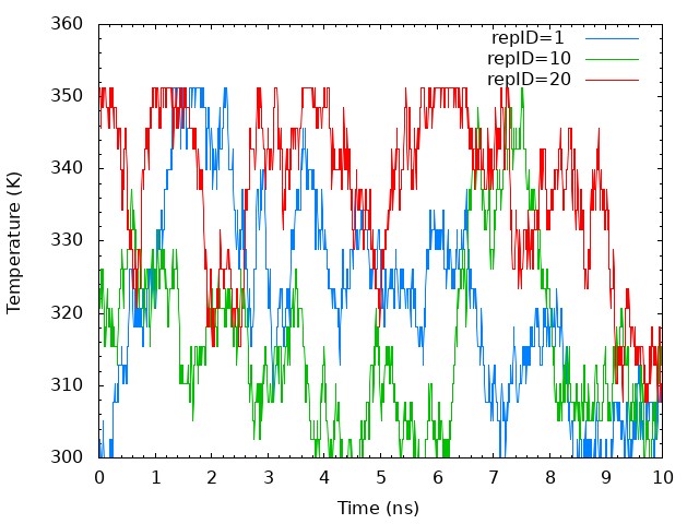
The temperatures of each replica during the simulation are distributed in all temperatures assigned. It means that correct annealing of the system is realized.

5.3. Sort coordinates in DCD trajectory files by parameters

The temperature in output DCD files of T-REMD simulation have all range of temperatures, due to the exchange. Therefore, to analyze the simulation further, we first need to sort the frames in the trajectory based on their temperature. To do that, we use GENESIS analysis tool remd_convert. Sorting is done based on the information written in remfiles generated from the REMD simulation. Concomitantly, we also sort log files for each replica based on temperature parameters

# change directory
$ cd ../3_sort
$ ls 
$ remd_convert.inp

# Sort frames by parameters
$ /home/user/GENESIS/bin/remd_convert remd_convert.inp | tee remd_convert.log 

The following control file is used to convert dcd files:

[INPUT]
psffile  = ../../1_setup/wbox.psf
reffile  = ../../1_setup/wbox.pdb
dcdfile  = ../../4_prod_remd/run_rep{}.dcd
remfile  = ../../4_prod_remd/run_rep{}.rem
logfile  = ../../4_prod_remd/run_rep{}.log

[OUTPUT]
pdbfile  = select.pdb
trjfile  = parmID{}.dcd
logfile  = parmID{}.log

[SELECTION]
group1           = segid:PROA
group2           = resno:2 and (an:N or an:CA or an:C or an:O)

[FITTING]
fitting_method   = TR+ROT
fitting_atom     = 2 
mass_weight      = YES

[OPTION]
check_only       = NO
convert_type     = PARAMETER
convert_ids      =              # (empty = all)
num_replicas     = 20
nsteps           = 4000000
exchange_period  = 2000
eneout_perio     = 2000
crdout_period    = 2000
trjout_format    = DCD 
trjout_type      = COOR+BOX
trjout_atom      = 1 
pbc_correct      = NO

Now we have sorted temperature log and DCD file which will be used in the following analysis steps.

5.4. Plot potential energy distribution for each temperature

Now as we already sorted the log files for each temperature parameters, we plot potential energy distribution to ensure sufficient overlap between all parameters. First, grep command we extract potential energies and step number, similar to previous plot of replica index.

# change directory
$ cd ../4_plot_potential
$ ls
$ plot_potential.sh plot_potential.gnuplot

# make the file executable and use it
$ chmod u+x plot_potential.sh
$ ./plot_potential.sh

# plot potential energy distribution 
gnuplot plot_potential.gnuplot

The file “plot_potential.sh” contains the following commands:

# get potential energies for each temperature
grep "INFO:" ../3_sort/remd_parmID1_trialanine.log   | tail -n +2 | awk '{print $2, $5}' > potential_energy_rep1.log
...
...
grep "INFO:" ../3_sort/remd_parmID20_trialanine.log  | tail -n +2 | awk '{print $2, $5}' > potential_energy_rep20.log

The file “plot_potential.gnuplot” contains the following commands:

set terminal jpeg
set output "pot-tempretures.jpg"
set key below
set xlabel "Potential Energy kcal/mol"
set ylabel "Probability"
binwidth=50
bin(x,width)=width*floor(x/width)
ndata=2000
plot for [k=1:20] "potential_parmID".k.".log" u (bin($2,binwidth)):(1.0/ndata) t "Tempreture".k with lines smooth freq

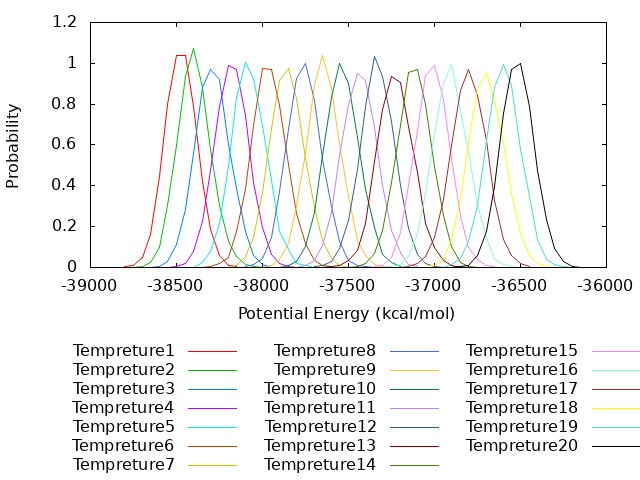
As can bee seen from the figure the potential energies of all temperatures have good overlap.

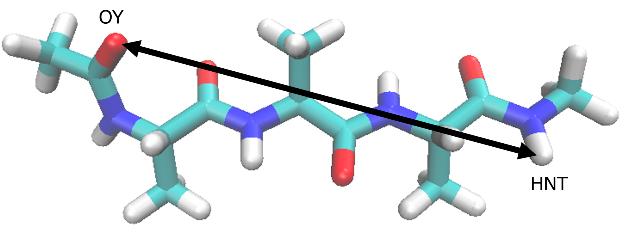
5.5. Calculating end to end distance

In order to calculate PMF (one dmension) of end to end distance distribution, in the current subsection we calculate the distance between the two terminal alanine (OY_HNT). In which we use GENESIS analysis tool trj_analysis as follow:

# change directory
$ cd ../5_end_end_distance
$ ls
$ generate_input_for_trj_analysis.sh  run_trj_end_to_end.sh

# make 20 input files
$ chmod u+x generate_input_for_trj_analysis.sh
$ ./generate_input_for_trj_analysis.sh

# run with 20 input files
$ chmod u+x run_trj_end_to_end.sh 
$ ./run_trj_end_to_end.sh

One created control file trj_end_end_parmID1.inp is used to calculate end to end distance as follow:

[INPUT]
psffile        = ../../1_setup/proa.psf
reffile        = ../../1_setup/proa.pdb

[OUTPUT]
disfile        = parmID1.dis

[TRAJECTORY]
trjfile1       = ../3_sort_dcd/parmID1.dcd
md_step1       = 4000000
mdout_period1  = 2000
ana_period1    = 2000
repeat1 = 1 
trj_format     = DCD       # (PDB/DCD)
trj_type       = COOR+BOX  # (COOR/COOR+BOX)
trj_natom      = 0         # (0:uses reference PDB atom count)

[OPTION]
check_only     = NO
distance1      = PROA:1:ALA:OY PROA:3:ALA:HNT

The file run_trj_end_to_end.sh include the following commands:

/home/user/GENESIS/trj_analysis trj_end_end_parmID1.inp | tee trj_end_end_parmID1.log
...
...
/home/user/GENESIS/trj_analysis trj_end_end_parmID20.inp | tee trj_end_end_parmID20.log

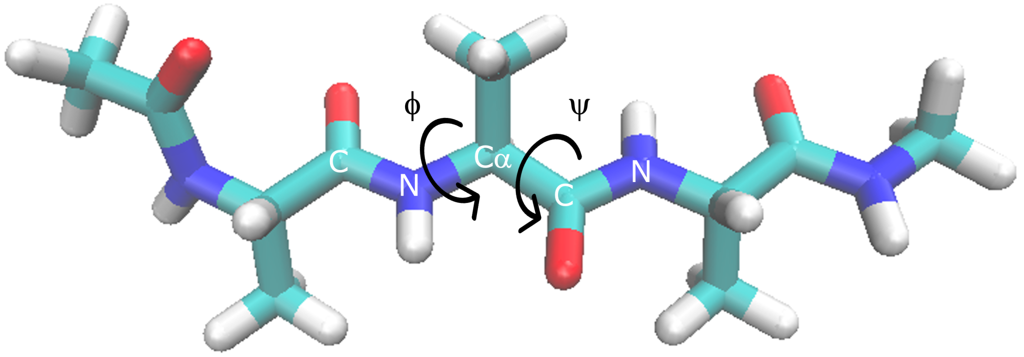
5.6. Calculating dihedral angle

In order to calculate PMF (two dimension) of dihedral angle distribution, in the current subsection we calculate two dihedral angle (Φ and Ψ) of 2nd alanine. As with end to end distance, we use GENESIS analysis tool trj_analysis as follow:

# change directory
$ cd ../6_dihedral_angle
$ ls
$ run_trj_dihedral.sh  trj_dihedral.sh

# make 20 input files
$ chmod u+x generate_input_for_trj_analysis.sh
$ ./trj_dihedral.sh

# run with 20 input files
$ chmod u+x run_trj_dihedral.sh 
$ ./run_trj_dihedral.sh

One created control file trj_dihedral_parmID1.inp is used to calculate end to end distance as follow:

[INPUT]
psffile        = ../../1_setup/proa.psf
reffile        = ../../1_setup/proa.pdb

[OUTPUT]
torfile        = parmID1.tor

[TRAJECTORY]
trjfile1       = ../3_sort_dcd/parmID1.dcd
md_step1       = 4000000
mdout_period1  = 2000
ana_period1    = 2000
repeat1 = 1 
trj_format     = DCD       # (PDB/DCD)
trj_type       = COOR+BOX  # (COOR/COOR+BOX)
trj_natom      = 0         # (0:uses reference PDB atom count)

[OPTION]
check_only     = NO
torsion1       = PROA:1:ALA:C PROA:2:ALA:N  PROA:2:ALA:CA PROA:2:ALA:C
torsion2       = PROA:2:ALA:N PROA:2:ALA:CA PROA:2:ALA:C  PROA:3:ALA:N

The file run_trj_dihedral.sh include the followind commands:

/home/user/GENESIS/trj_analysis trj_dihedral_parmID1.inp | tee trj_dihedral_parmID1.log
...
...
/home/user/GENESIS/trj_analysis trj_dihedral_parmID20.inp | tee trj_dihedral_parmID20.log

5.7. MBAR analysis

In order to use conformers from temperatures higher than the target temperature (300 K), we apply GENESIS mbar_analysis tool where we use our sorted potential energy files as cv as follows:

# change directory
$ cd ../7_MBAR
$ ls
$ MBAR.inp

# calculate free energy with MBAR
$ /home/user/GENESIS/bin/mbar_analysis MBAR.inp| tee MBAR.log 

The following control file MBAR.inp is used to calculate free energy:

[INPUT]
cvfile             = ../4_plot_potential/potential_parmID{}.log

[OUTPUT]
weightfile         = weight{}.dat
fenefile           = fene.dat

[MBAR]
num_replicas       = 20
input_type         = REMD
dimension          = 1 
temperature        = 300.00 302.53 305.09 307.65 310.24 \
                     312.85 315.47 318.12 320.78 323.46 \
                     326.16 328.87 331.61 334.37 337.14 \
                     339.94 342.75 345.59 348.44 351.30
target_temperature = 300.00
tolerance          = 10E-08
newton_iteration   = 100 
self_iteration     = 40

This produces fene.dat file containing the evaluated relative free energies and 20 weight*.dat files containing the weights of each snapshot for each parameterID. For example, weight1.dat is as follows:

        2000  2.792858134883802E-004
        4000  1.687935868689458E-004
...
...
     3998000  2.803355372323412E-004
     4000000  2.787713494107975E-004

5.8. Calculating PMF of distance distribution

The one of the final steps of this tutorial is to use the calculated distances (5.5). and weight files from MBAR analysis (5.7) to calculate PMF of end to end distance distribution in alanine tripeptide. We use another tool in GENESIS pmf_analysis as follow:

# change directory
$ cd ../8_PMF_distance
$ ls
$ PMF.inp plot_pmf.gnuplot

# calculate PMF
$ /home/user/GENESIS/bin/pmf_analysis PMF.inp| tee PMF.log 

# plot PMF 
$ gnuplot plot_pmf.gnuplot 

The following control file PMF.inp is used to calculate PMF about end to end distance:

[INPUT]
cvfile       = ../5_end_end_distance/parameter_ID{}.dis        # input cv file
weightfile   = ../6_MBAR/weight{}.dat

[OUTPUT]
pmffile      = dist.pmf

[OPTION]
nreplica     = 20         # number of replicas
dimension    = 1          # dimension of cv space
temperature  = 300 
grids1       = 0 15 61    # (min max num_of_bins)
band_width1  = 0.25       # sigma of gaussian kernel
                          # should be comparable or smaller than the grid size
                          # (pmf_analysis creates histogram by accumulating gaussians)
is_periodic1 = NO         # periodicity of cv1

The file plot_pmf.gnuplot include the following commands:

set terminal jpeg
set output "PMF_end_end.jpg"
set xrange [0:13]
set yrange [0:10]
set xlabel "End to End Distance (Å)"
set ylabel "PMF (kcal/mol)"
plot "dist.pmf" u 1:2 w l notitle

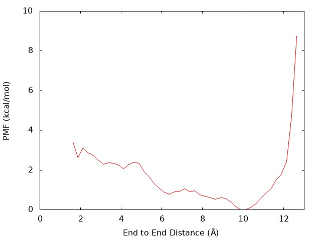
We can see that there is the global energy minimum around r = 10 Å. The latter corresponds to the α-helix conformation, where the hydrogen bond between OY and HNT is formed. These results suggest that in water the (Ala)₃ tends to form an extended conformation rather than α-helix.

5.9. Calculating PMF of dihedral distribution

The final step of this tutorial is to use the calculated dihedral angle (5.6) and weight files from MBAR analysis (5.7) to calculate PMF of dihedral distribution of 2nd alanine in (ALA)₃.

We can get PMF to the following commands:

# change directory 
$ cd ../9_PMF_dihedral 
$ ls 
$ calc_pmf_2d.py plot_pmf_2d.py

# merge data for python script
cp /dev/null cv.dat
cp /dev/null weight.dat
for i in {1..20}; do
cat ../6_dihedral_angle/parmID${i}.* >> cv.dat
cat ../7_MBAR/weight${i}.dat >> weight.dat
done

# calculate PMF
python3 calc_pmf_2d.py \
-t 300 \
-c 10 \
-n 40000 \
--Xmin -180 \
--Xmax 180 \
--Xdel 10 \
--Ymin -180 \
--Ymax 180 \
--Ydel 10 \
--cv_file cv.dat \
--weight_file weight.dat \
--out_file pmf_2d.dat \
--Xcyclic \
--Ycyclic

# print PMF
python3 plot_pmf_2d.py

Similar to the script of section 6.2 in Tutorial 13.1, the absolute temperature, the number of samples, the minimum value of the CV, the maximum value of the CV, the grid size of the bin for the CV are assigned by “-t”, “-n”, “–Xmin”, “–Xmax”, “–Xdel”, respectively. “-c” represents the cutoff of the number of samples in each bin. If the number of samples in a certain bin is below 10, the probability (or free energy) in the bin is omitted. “–Xcyclic” represents the periodicity of the CV. This script outputs the free energies in each bin “pmf.dat” and grid points of the CVs “xi.dat” and “yi.dat”. plot_pmf_2d.py draws the two-dimensional free-energy landscape using “pmf.dat”, “xi.dat”, and “yi.dat”.

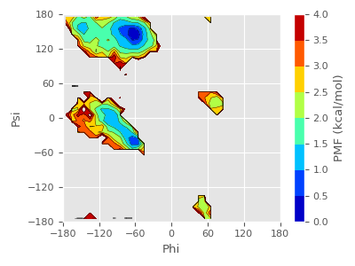
We can see that there is the global energy minimum around (φ,ψ) = (-75°, 150°) and local energy minimum around (φ,ψ) = (-60°, -45°). The latter corresponds to the PPII and α-helix conformation respectively. As in the PMF about end to end distance in (5.7), we can understand that (Ala)₃ in explicit water prefer extended conformation rather than α-helix.

References

Written by Daisuke Matsuoka@RIKEN Theoretical molecular science laboratory

Updated by Hisham Dokainish@RIKEN Theoretical molecular science laboratory
August, 28, 2019

Updated by Daiki Matsubara@RIKEN Center for Biosystems Dynamics Research (BDR)
March, 31, 2022

Y. Sugita et al., Chemical Physics Letters, 314, 141–151, (1999). ↩
J. E. basconi et al., J. Chem. Theory Comput. 9, 2887-2899, (2013). ↩
A. Patriksson et al, Phys. Chem. Chem. Phys., 10, 2073-2077, (2008). ↩
M. Shirts et al., J. Chem. Phys., 129, 124105-124114 (2008). ↩

REMD simulation of (Ala)3 in water