GENESIS Tutorial 11.4 (2022)
Coarse-grained MD simulation of FUS Condensation with the HPS model
Notice: This tutorial is for GENESIS v1.7.0 and later!
In this tutorial we will simulate the phase behavior of the low-complexity domain of the protein Fused in Sarcoma (FUS). This domain is intrinsically disordered and able to phase separate both in vivo and in vitro. Here we employ a recently developed CG model, the HPS 1, to simulate the dynamics of FUS with GENESIS.
0. Preparation
0.1 Install necessary softwares
Same as the other CG tutorials (tutorial 11.1, 11.2, 11.3), we have to first install the GENESIS-CG-tool 2 to generate CG coordinate and topology files.
0.2 Download the files for this tutorial
All the files required for this tutorial are hosted in the GENESIS tutorials repository on GitHub.
If you haven’t downloaded the files yet, open your terminal and run the following command (see more in Tutorial 1.1):
$ cd ~/GENESIS_Tutorials-2022

# if not yet
$ git clone https://github.com/genesis-release-r-ccs/genesis_tutorial_materials
If you already have the tutorial materials, let’s go to our working directory:
$ cd genesis_tutorial_materials/tutorial-11.4
This tutorial consists of two parts: 1) system setup and 2) MD simulations of FUS condensation:
$ ls
01_setup 02_simulation
1. Setup
As we mentioned above, here we focus on the intrinsically disordered region (IDR) in the protein FUS. Unlike the normal way to get “native” information from available PDB structures, we don’t have any reference structure for IDRs. Therefore, we will generate a straight initial conformation for the IDR. With the HPS model, we expect the IDR to relax and reach an equilibrium after sufficiently long simulation.
We prepared a file (fus.fasta) of the sequence of FUS:
$ cd 01_setup/
$ cat fus.fasta
> FUS WT
MASNDYTQQATQSYGAYPTQPGQGYSQQSSQPYGQQSYSGYSQSTDTSGYGQSSYSSYGQ
SQNTGYGTQSTPQGYGSTGGYGSSQSSQSSYGQQSSYPGYGQQPAPSSTSGSYGSSSQSS
SYGQPQSGSYSQQPSYGGQQQSYGQQQSYNPPQGYGQQNQYNS
We then use the GENESIS-CG-tool to create an artificial structure and topology files from this sequence:
$ /home/user/genesis_cg_tool/tools/modeling/protein_artifact/cg_protein_structure_builder.jl -s fus.fasta
This will generate five new files:
fus_cg.topandfus_cg.itp: CG topology files for the FUS IDR;fus_cg.gro: coordinate file for the FUS IDR;fus_cg.psf: PSF-style topology file for the FUS IDR;fus_cg.pdb: PDB file for the FUS IDR.
You may want to use a visualization software such as VMD or PyMOL to get
a glance of the initial structure, it looks like this:

2. MD simulations of FUS
2.1 Single chain
We first perform single-chain simulations of the FUS IDR to relax its conformation from the straight initial structure.
Let’s change the directory and copy necessary files:
$ cd ../02_simulation/02.1_single_chain/
$ ls
analysis/  param/ pro.inp

$ cp ../../01_setup/fus_cg.itp .
$ cp ../../01_setup/fus_cg.top .
$ cp ../../01_setup/fus_cg.gro .
In the directory we have already put a control file pro.inp:
[INPUT]
grotopfile = fus_cg.top
grocrdfile = fus_cg.gro

[OUTPUT]
pdbfile = fus_single_md1.pdb
dcdfile = fus_single_md1.dcd
rstfile = fus_single_md1.rst

[ENERGY]
forcefield = RESIDCG
electrostatic = CUTOFF
cg_cutoffdist_ele = 52.0
cg_cutoffdist_126 = 39.0
cg_pairlistdist_ele = 57.0
cg_pairlistdist_126 = 44.0
cg_sol_ionic_strength = 0.15
cg_IDR_HPS_epsilon = 0.2

[DYNAMICS]
integrator = VVER_CG
nsteps = 1000000
timestep = 0.010
rstout_period = 100000
crdout_period = 10000
eneout_period = 10000
nbupdate_period = 20

[CONSTRAINTS]
rigid_bond = NO

[ENSEMBLE]
ensemble = NVT
tpcontrol = LANGEVIN
temperature = 300
gamma_t = 0.01

[BOUNDARY]
type = NOBC
Compared with normal control files for CG simulations, here we have a new
variable, cg_IDR_HPS_epsilon, which controls the strength of the LJ potential.
In the param directory, the atom_types.itp file contains (line 126 to 211)
the parameters of the HPS potential. In the latest version of GENESIS-CG-tool,
these parameters default to a set proposed by Tesei et al. 3, but you can
change them to other published parameter sets 1, 2,
4 or any set of parameters you prefer. (Note that the developers of GENESIS
do not take any responsibility of changing parameters during the execution of MD
simulations.)
Now we can carry out the simulation with atdyn:
$ export OMP_NUM_THREADS=2
$ mpirun -np 4 /home/user/genesis/bin/atdyn pro.inp > fus_single_md1.log
This 106-step simulation will take several minutes on a laptop. After the simulation, four new files are created:
fus_single_md1.pdbis the final structure of the MD simulation;fus_single_md1.dcdis the MD trajectory;fus_single_md1.rstis the MD restarting file;fus_single_md1.logis the output of the time series of energies and other quantities.
2.1.1 Analysis of the MD trajectory of single-chain FUS
We are interested in the compactness of the FUS IDR. GENESIS provides a tool to calculate the radius-of-gyration (\(R_g\)). Here we use this tool to calculate the time series of \(R_g\) for FUS.
$ cd analysis
$ ls
rg_analysis.inp

$ /home/user/genesis/bin/rg_analysis rg_analysis.inp
After running the commands above, we will get a file output.rg, which contains
the \(R_g\) values of FUS at each frame in the MD trajectory. By
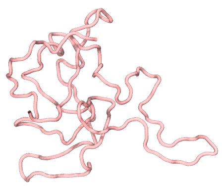
plotting \(R_g\) as a function of the simulation time, we can see that during
the 106-step run, the \(R_g\) of FUS quickly converges to a value
around 22Å. We can also use VMD or PyMOL to see the configuration of FUS stored
in the dcd file, which illustrates how the FUS collapsed from a straight line
(the initial structure) to a relatively compact conformation, as shown in the
following:
2.2 Multiple chains
We are going to duplicate the equilibrated single-chain FUS to construct the initial structure of the multiple FUS system. Now let’s change the directory and copy necessary files:
$ cd ../02.2_multiple_chains/
$ cp ../../01_setup/fus_cg.itp .
$ cp ../../01_setup/fus_cg.top .
$ cp ../02.1_single_chain/fus_single_md1.pdb .
The first step is to convert the PDB file we got in the MD simulation of single FUS into the grocrd format. We can do this with the GENESIS-CG-tool:
$ /home/user/genesis_cg_tool/tools/fileformat_conversion/pdb_2_gro.jl -t fus_cg.top -p fus_single_md1.pdb --pdb-noTER -o fus_single.gro
This command reads information from fus_single_md1.pdb and writes the
coordinates into fus_single.gro.
We then use another script in the GENESIS-CG-tool to create duplications of the single FUS:
$ /home/user/genesis_cg_tool/tools/modeling/duplication_modeling/duplication_generator.jl -t fus_cg.top -c fus_single.gro -o fus_cg --nx 2 --ny 2 --nz 30
System name:fus_cg
Number of particles in top:163
Duplicated system has 2 x 2 x 30 x 100% = 120 copies, in total 19560 atoms
Duplicated system size: 125.990 x 122.242 x 1773.420
Now we have a new system (fus_cg_mul_2_2_30_n_120.gro) composing of 2
× 2 × 30 = 120 copies of the single FUS and the (estimated) system size
was 125.999 × 122.142 × 1773.420 Å3. In real simulation, we need to
set the PBC box size larger than this one. Besides, don’t forget to make
changes to the topology file (here we create a new file fus_cg_120.top):
$ cp fus_cg.top fus_cg_120.top
$ vim fus_cg_120.top
...

$ cat fus_cg_120.top
#include "./param/atom_types.itp"
#include "./param/flexible_local_angle.itp"
#include "./param/flexible_local_dihedral.itp"
#include "./param/pair_energy_MJ_96.itp"

#include "fus_cg.itp"

[ system ]
multiple fus_cg

[ molecules ]
fus_cg 120

[ cg_ele_chain_pairs ]
ON 1 - 120 : 1 - 120
As can be seen, we have 120 “fus_cg” chains as assigned in the [ molecules ]
block. We also want to calculate electrostatic interactions among all the 120
chains, as described in the [ cg_ele_chain_pairs ].
The control file for the 120-FUS simulation (fus_120.inp) looks like
this:
[INPUT]
grotopfile = fus_cg_120.top
grocrdfile = fus_cg_mul_2_2_30_n_120.gro

[OUTPUT]
pdbfile = fus_120_run.pdb
dcdfile = fus_120_run.dcd
rstfile = fus_120_run.rst

[ENERGY]
forcefield = RESIDCG
electrostatic = CUTOFF
cg_cutoffdist_ele = 52.0
cg_cutoffdist_126 = 39.0
cg_pairlistdist_ele = 57.0
cg_pairlistdist_126 = 44.0
cg_sol_ionic_strength = 0.15
cg_IDR_HPS_epsilon = 0.2

[DYNAMICS]
integrator = VVER_CG
nsteps = 10000000
timestep = 0.010
rstout_period = 1000000
crdout_period = 10000
eneout_period = 10000
nbupdate_period = 20

[CONSTRAINTS]
rigid_bond = NO

[ENSEMBLE]
ensemble = NVT
tpcontrol = LANGEVIN
temperature = 300
gamma_t = 0.01

[BOUNDARY]
type = PBC
box_size_x = 180.0
box_size_y = 180.0
box_size_z = 1800.0
As mentioned earlier, the simulation box size is slightly larger than the initial duplicated system, and the shape is a “slab” that the z-dimension is much larger than the other two.
Now let’s run the simulation with atdyn:
$ export OMP_NUM_THREADS=2; mpirun -np 4 ~/Workspace/genesis/bin/atdyn fus_120.inp > fus_120_run.log
After the simulation, you can use your favorite visualization tool to take a look at the MD trajectory. The final structure of the 120 FUS may look like this:

Note that due to the randomness of Langevin dynamics, your final structure may looks different. For example, the FUS chains may aggregate into two or more smaller clusters.
Written by Cheng Tan@RIKEN Center for Computational Science, Computational Biophysics Research Team, October, 2021
References
-
Dignon G. L., Zheng W., Kim Y. C., Best R. B., Mittal J., PLOS Comput. Biol., 2018, 14(1), e1005941. ↩ ↩2
-
Regy, R. M., Thompson, J., Kim, Y. C. & Mittal, J. 2021, Protein Sci 30, 1371–1379. ↩ ↩2
-
Tesei, G., Schulze, T. K., Crehuet, R. & Lindorff-Larsen, K. 2021, Proc National Acad Sci 118, e2111696118. ↩
-
Dannenhoffer-Lafage T. and Best R. B., 2021, J Phys Chem B 125(16), 4046–4056. ↩