GENESIS Tutorial 11.3 (2022)
Coarse-grained MD simulation of TBP-DNA Sequence-Specific Recognition
Notice: This tutorial is for GENESIS v1.7.0 and later!
In this tutorial we will simulate the specific recognition of a special DNA sequences, the “TATA-box”, by the TATA-box binding protein (TBP). TBP is a general transcription factor that participates in the initialization of transcription. It uses a beta-sheet surface to bind to the minor groove of DNA and induces sharp bending of DNA. Here we will use the AICG2+ model1 for TBP and the 3SPN.2C model2 for DNA. For intermolecular protein-DNA interactions, we consider excluded-volume, electrostatics, and sequence-specific interactions. Particularly, the last one is modeled by the PWMcos method.3
0. Preparations
0.1 Install necessary softwares
Same as in tutorial 11.1 and 11.2, we will use the GENESIS-CG-tool 4 to generate CG coordinate and topology files.
0.2 Download the files for this tutorial
All the files required for this tutorial are hosted in the GENESIS tutorials repository on GitHub.
If you haven’t downloaded the files yet, open your terminal and run the following command (see more in Tutorial 1.1):
$ cd ~/GENESIS_Tutorials-2022

# if not yet
$ git clone https://github.com/genesis-release-r-ccs/genesis_tutorial_materials
If you already have the tutorial materials, let’s go to our working directory:
$ cd genesis_tutorial_materials/tutorial-11.3
This tutorial consists of two parts: 1) system setup; and 2) MD simulations of TBP binding on DNA:
$ ls
01_setup 02_simulation
1. Setup
1.1 Prepare the DNA structure and topology
Let’s go to our working directory:
$ cd 01_setup
$ ls
dsDNA.fasta
Here we want to simulate the binding of TBP on a 50bp dsDNA. The DNA
sequence file dsDNA.fasta looks like this:
> dsDNA for TBP binding
AGCAATTAGCCAGGGAATGTATAAAAGGCGTCAGGGAGACTCACTGGGCT
Here we will prepare the DNA topology and coordinate files in the same way as in tutorial 11.2:
$ /home/user/genesis_cg_tool/tools/modeling/DNA_general/build_dna.jl -s dsDNA.fasta -C -o dsDNA
Please refer to tutorial 11.2 for more details of generating DNA CG files.
1.2 Prepare the protein topology files
Now let’s download the PDB file from RCSB:
$ wget https://files.rcsb.org/download/1CDW.pdb
We first make a copy of the PDB file and do some modification so that it contains only the protein.
$ grep -E "^ATOM.{17}A" 1CDW.pdb > tbp.pdb
$ echo "END" >> tbp.pdb
Now let’s generate the CG topology and coordinate fils for TBP:
$ /home/user/genesis_cg_tool/src/aa_2_cg.jl tbp.pdb
We will get several new files: tbp_cg.gro, tbp_cg.top, and tbp_cg.itp. The
first one is the coordinate file for TBP, and the later two are the topology
files.
So far we have finished the preparation for the DNA and the protein, respectively. The commands have been also introduced in tutorial 11.1 and 11.2. However, these files are not enough to study the specific recognition between TBP and DNA. In the next section we will show how to prepare the sequence-specific interaction parameters.
1.3 Introduce sequence specificity
In the PWMcos model, sequence specificity is described by the position weight matrix (PWM). However, very often another form, the position frequency matrix (PFM), is provided by experiments. The PFMs are deposited on databases like JASPAR and UniPROBE. Now let’s download the PFM from the TBP entry on JASPAR.
$ wget http://jaspar.genereg.net/api/v1/matrix/MA0108.1.jaspar
The PFM file for TBP looks like this:
> MA0108.1 TBP
A [  61  16 352   3 354 268 360 222 155  56  83  82  82  68  77 ]
C [ 145  46   0  10   0   0   3   2  44 135 147 127 118 107 101 ]
G [ 152  18   2   2   5   0  10  44 157 150 128 128 128 139 140 ]
T [  31 309  35 374  30 121   6 121  33  48  31  52  61  75  71 ]
Each element in the matrix represents the frequency of a base type (“A”, “C”, “G”, or “T”) appearing at a position. The matrix also shows the “consensus sequence”, which is the most probable target sequence. Based on the PFM above, the consensus sequence for TBP is: “GTATAAAAGGCGGGG”.
The PWMcos model incorporates the PFM and the protein-DNA binding structural information based on the PDB structure. For the model to work, we have to match up the consensus sequence with the DNA sequence in the TBP-DNA complex PDB structure (1CDW). Note that for some proteins the available PDB DNA sequence can be different from the PFM consensus sequence. Therefore, we have to add the sequence index information into the PFM file, and then use our GENESIS-CG-tool to extract CG parameters.
Let’s first use the GENESIS-CG-tool to get the sequence information from “1CDW.pdb”:
$ /home/user/genesis_cg_tool/src/aa_2_cg.jl 1CDW.pdb --show-sequence
This command generates a new file, 1CDW_cg.fasta, which lists the
sequence of dsDNA and TBP:
> Chain A : DNA
CTGCTATAAAAGGCTG
> Chain B : DNA
CAGCCTTTTATAGCAG
> Chain C : protein
SGIVPQLQNIVSTVNLGCKLDLKTIALRARNAEYNPKRFAAVIMRIREPRTTALIFSSGKMVCTGAKSEENSRLAARKYARVVQKLGFPAKFLDFKIQNMVGSCDVKFPIRLEGLVLTHQQFSSYEPELFPGLIYRMIKPRIVLLIFVSGKVVLTGAKVRAEIYEAFENIYPILKGFRK
For clarity, here we align the PFM consensus sequence and the sequence
of chain A in the PDB, as shown below:
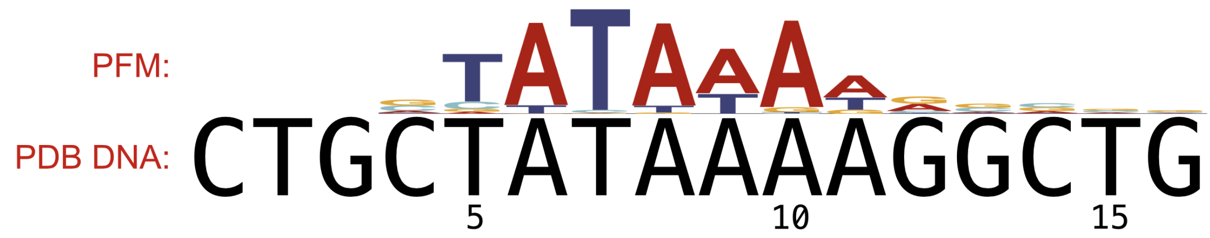
As can be seen in the figure, the “TATAAAAG” motif matches a segment of “Chain A”. We then add the indices of each base to a new “PFM” file:
$ cp MA0108.1.jaspar tbp.pfm
$ vim tbp.pfm
...
This is the content of the new file tbp.pfm:
$ cat tbp.pfm
A       61  16 352   3 354 268 360 222 155  56  83  82  82
C      145  46   1  10   1   1   3   2  44 135 147 127 118
G      152  18   2   2   5   1  10  44 157 150 128 128 128
T       31 309  35 374  30 121   6 121  33  48  31  52  61
CHAIN_A  4   5   6   7   8   9  10  11  12  13  14  15  16
CHAIN_B 29  28  27  26  25  24  23  22  21  20  19  18  17
Compared with the original PFM file, we added two more lines, “CHAIN_A” and “CHAIN_B”, listing the indices of each base (in CHAIN_A) and its complementary base (in CHAIN_B) in the PDB file, respectively. Let’s take column 3 (16, 46, 18, 309, 5, and 28) as an example, the first four elements, 16, 46, 18, and 309 show the frequency of each base type appearing at this position, from which we can tell that the most probable base-pair at this position is “T-A”. Correspondingly, the last two elements in this column, 5 and 28, describe the residue indices of the “T” and “A” in PDB, respectively. Note that some elements in the PFM are changed from “0” to “1” (for instance, row 2 column 3 of base type “C”). This is because in the transition from PFM to PWM, we have to take the logarithm of each element of the PFM. Therefore, we replace all the “0”s in the PFM with some small “pseudo counts”.5
It’s time to run the GENESIS-CG-tool again:
$ /home/user/genesis_cg_tool/src/aa_2_cg.jl 1CDW.pdb --pwmcos -p tbp.pfm --patch tbp_cg.itp --pwmcos-scale 3.9 --pwmcos-shift -0.4
Here the --pwmcos option tell the program to generate parameters for the
PWMcos model, -p specifies the PFM file, and the --patch option is used to
tell GENESIS-CG-tool to append information to the .itp file, instead of writing
a new file. The options --pwmcos-scale and --pwmcos-shift are used to
specify energy scaling and shifting factor parameters (see reference 3).
Let’s take a look at the PWMcos information added to the end of tbp_cg.itp:
$ tail -n 34 tbp_cg.itp

[ pwmcos ]
;    i   f       r0   theta1   theta2   theta3       ene_A       ene_C       ene_G       ene_T   gamma    eps'
     9   1  0.84956   57.727   50.211   73.212   -0.549774    0.649174    0.649174   -0.748573   3.900  -0.400
     9   1  0.71936   43.555   90.626  100.377   -0.136243    0.222109    0.543997   -0.629863   3.900  -0.400
    11   1  0.73831   74.045   74.387   97.686   -0.748573    0.649174    0.649174   -0.549774   3.900  -0.400
    11   1  0.77045   77.501  119.188   66.900   -0.779085    0.417788    0.116795    0.244501   3.900  -0.400
    11   1  0.84433   73.607   95.508  117.177   -0.549774    0.649174    0.649174   -0.748573   3.900  -0.400
    39   1  0.89446   88.977   80.059   46.823   -0.698333    0.560902   -0.711154    0.848584   3.900  -0.400
    39   1  0.85164   40.710  110.258   82.867   -0.225368   -0.023048    0.595161   -0.346745   3.900  -0.400
    54   1  0.86112   71.731   96.581   78.999   -0.346745    0.595161   -0.023048   -0.225368   3.900  -0.400
    54   1  0.99176   73.711   62.729   97.297   -0.225368   -0.023048    0.595161   -0.346745   3.900  -0.400
    54   1  0.91174   51.774  103.448  119.680    0.244501    0.116795    0.417788   -0.779085   3.900  -0.400
    56   1  0.96820   45.851   62.446  117.385   -0.346745    0.595161   -0.023048   -0.225368   3.900  -0.400
    62   1  0.77175   67.992   66.006   78.669   -0.779085    0.417788    0.116795    0.244501   3.900  -0.400
    62   1  0.76489   57.497  120.218  106.229   -0.346745    0.595161   -0.023048   -0.225368   3.900  -0.400
    64   1  0.83361   65.631   49.092   92.389    0.244501    0.116795    0.417788   -0.779085   3.900  -0.400
    99   1  0.82029   62.630   44.493   70.209   -0.629863    0.543997    0.222109   -0.136243   3.900  -0.400
    99   1  0.70661   46.042   94.654   97.889   -0.748573    0.649174    0.649174   -0.549774   3.900  -0.400
   101   1  0.80936   83.242   91.310  115.240   -0.629863    0.543997    0.222109   -0.136243   3.900  -0.400
   101   1  0.82360   68.789   70.757   94.587   -0.136243    0.222109    0.543997   -0.629863   3.900  -0.400
   101   1  0.79289   73.791  122.905   66.823   -0.854901    0.452876    0.050516    0.351509   3.900  -0.400
   130   1  0.72926   67.554   60.872  100.415    0.344549   -0.007469    0.305288   -0.642368   3.900  -0.400
   130   1  0.74848   52.461  124.421   80.672   -0.833900    0.632008    0.458721   -0.256829   3.900  -0.400
   130   1  0.76783   82.299   69.256   56.852   -0.642368    0.305288   -0.007469    0.344549   3.900  -0.400
   131   1  0.75497   52.985   75.962  100.165   -0.642368    0.305288   -0.007469    0.344549   3.900  -0.400
   145   1  0.89136   82.196   55.199   90.577   -0.833900    0.632008    0.458721   -0.256829   3.900  -0.400
   145   1  0.87418   57.042  107.171  117.041    0.351509    0.050516    0.452876   -0.854901   3.900  -0.400
   145   1  0.89606   63.280  101.351   75.223   -0.256829    0.458721    0.632008   -0.833900   3.900  -0.400
   147   1  0.99519   38.996   72.000  112.916   -0.256829    0.458721    0.632008   -0.833900   3.900  -0.400
   153   1  0.73206   65.505   67.541   78.456   -0.854901    0.452876    0.050516    0.351509   3.900  -0.400
   155   1  0.84186   64.475   49.574   92.180    0.351509    0.050516    0.452876   -0.854901   3.900  -0.400
   155   1  0.69313   53.556   98.903   66.205   -0.629863    0.543997    0.222109   -0.136243   3.900  -0.400
Please refer to the wiki-page of the GENESIS-CG-tool for the meaning of each column.
2. MD simulation of TBP Binding and Induced Bending of DNA
Let’s go to the working directory to carry out MD simulations:
$ cd 02_simulation
$ ls
pro_dna.inp tbp_dna.top tbp_dna_init.gro
2.1 The control file
This is the content of the control file pro_dna.inp:
[INPUT]
grotopfile = tbp_dna.top
grocrdfile = tbp_dna_init.gro

[OUTPUT]
pdbfile = pro_dna_test_run.pdb
dcdfile = pro_dna_test_run.dcd
rstfile = pro_dna_test_run.rst

[ENERGY]
forcefield = RESIDCG
electrostatic = CUTOFF
cg_cutoffdist_ele = 52.0
cg_cutoffdist_DNAbp = 18.0
cg_pairlistdist_ele = 57.0
cg_pairlistdist_PWMcos = 23.0
cg_pairlistdist_DNAbp = 23.0
cg_pairlistdist_exv = 15.0
cg_sol_ionic_strength = 0.15
cg_pro_DNA_ele_scale_Q = -1.0

[DYNAMICS]
integrator = VVER_CG
nsteps = 3000000
timestep = 0.010
rstout_period = 100000
crdout_period = 10000
eneout_period = 10000
nbupdate_period = 100
stoptr_period = 100

[CONSTRAINTS]
rigid_bond = NO

[ENSEMBLE]
ensemble = NVT
tpcontrol = LANGEVIN
temperature = 300
gamma_t = 0.01

[BOUNDARY]
type = NOBC
Most of the options have been already explained in tutorial
11.1 and
11.2. Specifically, here we have one
more “pairlistdist” option for the PWMcos: cg_pairlistdist_PWMcos.
Notably, the charge of phosphate in the 3SPN.2C model is set to -0.6e (for
electrostatics between DNA particles). However, in protein-DNA interactions we
use a value of -1.0e, considering the effect of counter-ion redistribution 3, 6. Therefore, here we set a new value for the phosphate charge in the
electrostatic interactions between protein and DNA to be
cg_pro_DNA_ele_scale_Q = -1.0.
2.2 The topology file
In the same directory we also provided the topology file (tbp_dna.top)
for the protein-DNA complex:
#include "./param/atom_types.itp"
#include "./param/flexible_local_angle.itp"
#include "./param/flexible_local_dihedral.itp"
#include "./param/pair_energy_MJ_96.itp"

; Molecule topologies
#include "./top/dsDNA_cg.itp"
#include "./top/tbp_cg.itp"

[ system ]
TBP-DNA specific interactions

[ molecules ]
dsDNA_cg  1
tbp_cg    1

[ cg_ele_chain_pairs ]
ON 1 - 3 : 1 - 3
OFF 3 - 3

[ pwmcos_chain_pairs ]
ON 1 - 2 : 3 - 3
The first four lines import the general parameters. Then in line 7 and 8 we include the topology files for DNA and TBP, respectively.
Now let’s copy the necessary .itp files to the subdirectory top/:
$ mkdir top/
$ cp ../01_setup/dsDNA_cg.itp top/
$ cp ../01_setup/tbp_cg.itp top/
Let’s go back to the tbp_dna.top. In the [ system ] block we specify the
name for the system. Importatnly, in the [ molecules ] block, we assign the
name and the number of each molecule. Note that the molecule names listed here
should be the same as the ones written in the [ moleculetype ] block of the
“.itp” files. For instance, we can print out the molecule name of the dsDNA in
the dsDNA_cg.itp:
$ head -n 3 top/dsDNA_cg.itp
[ moleculetype ]
;name nrexcl
dsDNA_cg 3
As can be seen, the name of dsDNA is the same as the one we write in the
tbp_dna.top.
Besides, the order of molecules in the [ molecules ] block should be the same
as the order of molecules in the coordinate file (“tbp_dna_init.gro”,
described in the next section).
There are two more blocks describing the inter-molecular interactions, namely,
the “[ cg_ele_chain_pairs ]” and the “[ pwmcos_chain_pairs ]”. In the “[
cg_ele_chain_pairs ]” we first turn on all the intra- and inter-molecular
electrostatics in the system, then turn off the intra-molecular electrostatic
interactions in the TBP (chain No. 3). Similarly, in the “[ pwmcos_chain_pairs
]”, we assign the PWMcos interactions between DNA (chains No. 1 and 2) and the
TBP (chain No. 3). You can find more explanations at the wiki-page of the
GENESIS-CG-tool.
2.3 The coordinate file
The tbp_dna_init.gro file contains all the coordinates of DNA and TBP. The
initial structure was taken from a structure reported in reference 3. In this
structure TBP has already found its consensus sequence on DNA, and the DNA is
bent to an extent similar to the PDB structure. You can start from a dissociated
state, but it may take a long time for the TBP to find its target on DNA.
Therefore, here we simply start from the bound state.
2.4 Run simulation
Now let’s execute atdyn:
$ export OMP_NUM_THREADS=2
$ mpirun -np 4 /home/user/GENESIS/bin/atdyn pro_dna.inp > pro_dna_test_run.log
This simulation will create the following new files:
pro_dna_test_run.dcd: MD trajectory file;pro_dna_test_run.pdb: PDB structure of the last frame;pro_dna_test_run.rst: MD restarting file;pro_dna_test_run.log: GENESIS log file for MD simulation.
You can use VMD or other MD visualization software to take a look at the
structure (pro_dna_test_run.pdb) or the trajectory (pro_dna_test_run.dcd).
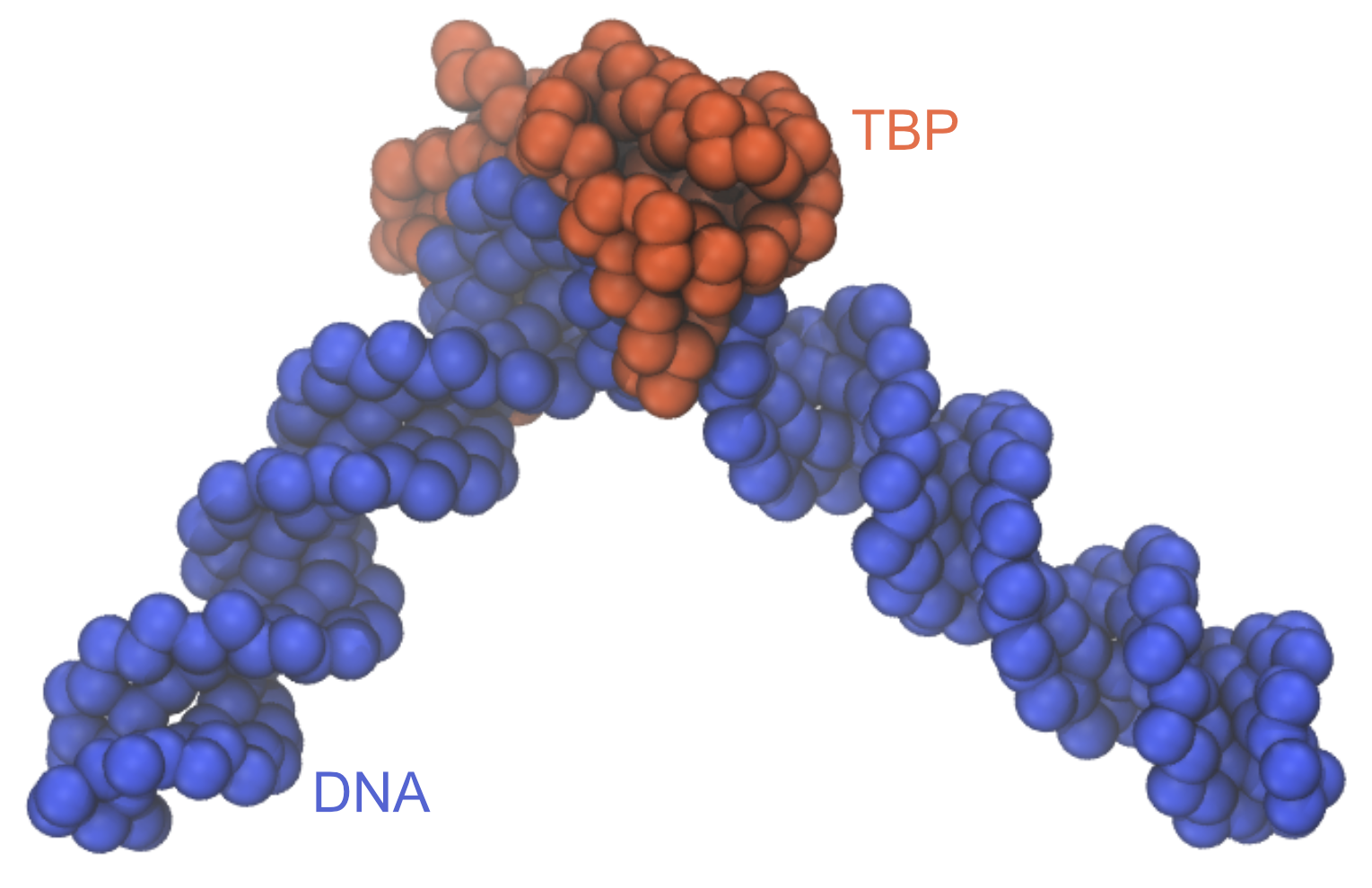
The structure of the TBP-DNA complex looks like this:
Written by Cheng Tan@RIKEN Center for Computational Science, Computational Biophysics Research Team, October, 2021
References
-
Li W., Wang W., Takada S., 2014, Proc. Nation. Acad. Sci., 111, 10550-10555. ↩
-
Freeman G. S., Hinckley D. M., Lequieu J. P., Whitmer J. K., de Pablo J. J., 2014, J. Chem. Phy., 141 (16), 165103. ↩
-
Tan C., Takada S., 2018, J. Chem. Theor. Comput., 14, 3877-3889. ↩ ↩2 ↩3 ↩4
-
Tan C., Jung J., Kobayashi C., Ugarte La Torre D., Takada S., and Sugita Y., 2022, PLoS Computational Biology 18(4), e1009578. ↩
-
Keishin Nishida, Martin C. Frith, Kenta Nakai, 2009, Nucleic Acids Research, 37 (3), 939–944. ↩
-
Lequieu J., Cordoba A., Schwartz D. C., de Pablo J. J., 2016, ACS Cent. Sci., 2, 660-666. ↩