GENESIS Tutorial 11.1 (2022)
Coarse-grained MD simulation of protein with the AICG2+ model
Notice: This tutorial is for GENESIS v1.7.0 and later!
The atomic interaction-based coarse-grained model version 2+ (AICG2+)1 is a refined version of the classic Gō-model2 for proteins. In this model, each amino acid is represented by a single CG particle.
In this tutorial, we demonstrate how to simulate a small protein using the AICG2+ model in GENESIS. We will walk through the complete process—from system setup to basic analysis of the simulation results.
0. Preparations
0.1. Download GENESIS-cg-tool for Preparing CG Simulation Files
To begin, we need a set of scripts that assist in generating the topology and coordinate files required for CG MD simulations in GENESIS. This collection of scripts is referred to as the GENESIS-cg-tool.3
The tool is included in the GENESIS package and can be found in the
src/analysis/cg_tools subdirectory. Alternatively, it is available on
GitHub,
and can be downloaded using git:
$ git clone https://github.com/genesis-release-r-ccs/genesis_cg_tool
This tool is developed using the Julia programming language. Before using it, please make sure to:
- Install Julia on your system.
- Learn some basic operations in Julia if you are not already familiar with the language.
- Install the required Julia package
ArgParse, which is a dependency of the GENESIS-cg-tool.
You can install ArgParse by launching Julia and running:
$ julia
julia> import Pkg
julia> Pkg.add("ArgParse")
Alternatively, you can also execute the following command to install all dependencies:
$ /home/user/genesis_cg_tool/opt/dependency.jl
Remember that you can always find the help information of the GENESIS-cg-tool by running:
$ /home/user/genesis_cg_tool/src/aa_2_cg.jl -h
0.2. Download files for this tutorial
All the files required for this tutorial are hosted in the GENESIS tutorials repository on GitHub.
If you haven’t downloaded the files yet, open your terminal and run the following command (see more in Tutorial 1.1):
$ cd ~/GENESIS_Tutorials-2022

# if not yet
$ git clone https://github.com/genesis-release-r-ccs/genesis_tutorial_materials
If you already have the tutorial materials, let’s go to our working directory:
$ cd genesis_tutorial_materials/tutorial-11.1
This tutorial is divided into three major steps: 1) System Setup; 2) MD Simulation; and 3) Trajectory Analysis.
$ ls
01_setup 02_simulation 03_analysis
1. Setup
We get started from preparing the topology and coordinate files for the system. Unlike atomistic simulations, we cannot simply download the PDB file and make use of some standard force-field files. Instead, we have to generate all the files by ourselves, which can be easily done with the help of the GENESIS-cg-tool.
As an example, we download a pdb file of protein GB1 from the RCSB:
$ cd 01_setup
$ wget https://files.rcsb.org/download/1PGB.pdb
We then use the GENESIS-cg-tool to extract information from the pdb file and generate the CG files:
$ /home/user/genesis_cg_tool/src/aa_2_cg.jl 1PGB.pdb
$ ls
1PGB.pdb 1PGB_cg.gro 1PGB_cg.itp 1PGB_cg.top
Don’t forget to change “/home/user/genesis_cg_tool” in the command
above to your real path of the GENESIS-cg-tool.
The 1PGB_cg.gro file contains the coordinates of the CG particles.
The 1PGB_cg.itp file defines the parameters for interactions
including bonds, angles, dihedral angles, and native contacts.
The main topology file, 1PGB_cg.top, incorporates these parameters using
#include directives, referencing both the 1PGB_cg.itp and other standard
parameter files.
For a detailed explanation of the topology file format, please refer to the GENESIS-CG-tool wiki.
You can add more options to the aa_2_cg.jl command:
$ /home/user/genesis_cg_tool/src/aa_2_cg.jl 1PGB.pdb --psf --cgpdb
$ ls
1PGB.pdb 1PGB_cg.gro 1PGB_cg.itp 1PGB_cg.pdb 1PGB_cg.psf 1PGB_cg.top
The two extra files, 1PGB_cg.psf and 1PGB_cg.pdb, are not necessary for
running MD simulations. However, you many want to use them in some structure
visualization softwares. Importantly, this simplified “psf” file does not have
enough information about the interaction terms, please always consider using the
grotop and groitp files for simulations and analysis.
Now, you can check the CG pdb file with VMD:
$ vmd 1PGB_cg.pdb
Change the representation to “VDW” to view the CG particles as spheres. In the following figure, we set the color of each particle according to its index. To see the same coloring effect, please change the “Coloring Method” to “Index” in VMD.
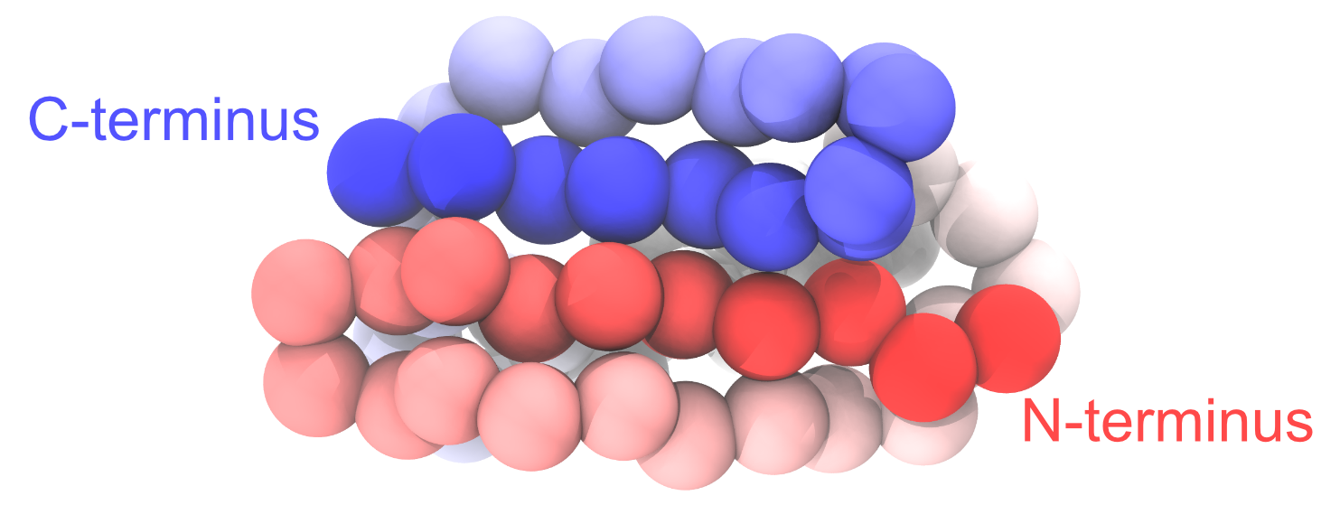 Figure: Coarse-grained protein generated from PDB 1PGB.
2. MD simulations
Now let’s move to the simulation working directory:
$ cd 02_simulation
$ ls
param/   pro.inp
In the param/ directory there are standard parameter files (you can find a
copy from the GENESIS-cg-tool). The file pro.inp is the control file that
contains the information for Genesis to perform the MD simulation. Let’s take a
look at it:
[INPUT]
grotopfile = 1PGB_cg.top # topology file
grocrdfile = 1PGB_cg.gro # coordinate file

[OUTPUT]
pdbfile = pro_md1.pdb # PDB output
dcdfile = pro_md1.dcd # DCD trajectory
rstfile = pro_md1.rst # restart file

[ENERGY]
forcefield          = RESIDCG # Residue-level CG models
electrostatic       = CUTOFF  # Debye-Huckel model
cg_pairlistdist_exv = 15.0    # Neighbor-list distance

[DYNAMICS]
integrator      = VVER_CG  # velocity-verlet propagation
nsteps          = 50000000 # number of MD steps
timestep        = 0.010    # timestep size (ps)
eneout_period   = 10000    # energy output interval
crdout_period   = 10000    # trajectory output interval
rstout_period   = 100000   # restart output interval
nbupdate_period = 20       # pairlist update interval

[CONSTRAINTS]
rigid_bond = NO        # don't apply constraints

[ENSEMBLE]
ensemble    = NVT      # Canonical ensemble
tpcontrol   = LANGEVIN # Langevin thermostat
temperature = 400      # simulation temperature
gamma_t     = 0.01     # thermostat friction parameter

[BOUNDARY]
type       = PBC   # periodic boundary condition
box_size_x = 180.0 # box size in x direction
box_size_y = 180.0 # box size in y direction
box_size_z = 180.0 # box size in z direction
The control file contains several sections, such as [INPUT],
[OUTPUT], and [ENERGY], where we can specify the options for the
simulation.
- In the
[INPUT]section, we set the file names for the topology file (1PGB_cg.top) and the coordinate file (1PGB_cg.gro). As described above,1PGB_cg.topis the main topology file and it links the information of1PGB_cg.itp. - In the
[OUTPUT]section, output filenames are set. Atdyn does not create any output file unless we explicitly specify their names. Particularly, the “pdb” file contains the coordinates of the last snapshot of the simulation; the “dcd” file is the MD trajectory; and the “rst” file contains the information for restarting a simulation. - In the
[ENERGY]section, we specify the parameters related to the energy and force evaluation. RESIDCG is the name for the residue-level coarse-grained models in GENESIS. Here we also set the pair-list distance for the non-native contacts (represented by the excluded volume potentialcg_pairlistdist_exv). You can consider different values to balance computational efficiency and accuracy. As for the native contacts, all the interaction energies are calculated in GENESIS, without any cutoff. - The
[DYNAMICS]section sets up the parameters for the MD engine ofatdyn. Specifically for CG simulations, GENESIS provides a high-efficiency integrator, “VVER_CG”. For the AICG2+ model, time step (timestep) can be set to 10 fs. The total number of steps (nsteps) is50000000in this example, but you may want to change it to a smaller value if you are carrying out the simulations on your laptop. - In the
[CONSTRAINTS]section, we disable all constraints (rigid_bond=NO). - In the
[ENSEMBLE]section, the LANGEVIN thermostat is chosen for an isothermal simulation with the friction constant of 0.01 ps-1. - Finally, in the
[BOUNDARY]section, we set the boundary conditions for the system. Generally speaking, we don’t have to worry about the computational efficiency when choosing the box size, since there are no water molecules filling the space. However, please make the box length in each dimension larger than 3 times the longestpairlistdist(57Å for the electrostatic interactions by default).
Now let’s copy necessary files prepared in the previous step:
$ cp ../01_setup/1PGB_cg.top .
$ cp ../01_setup/1PGB_cg.gro .
$ cp ../01_setup/1PGB_cg.itp .
Finally, we can run GENESIS atdyn:
$ export OMP_NUM_THREADS=2
$ mpirun -np 4 /home/user/GENESIS/bin/atdyn pro.inp > pro_md1.log
The 50000000-step simulation takes about half an hour on our PC cluster.
You may want to decrease “nsteps” to save some time in your test.
Once the simulation finishes, we will get four new files:
pro_md1.dcd: MD trajectory filepro_md1.pdb: PDB file of the last snapshotpro_md1.rst: MD restart filepro_md1.log: MD information log
In the pro_md1.log file you can check the potential energy values of each
interaction term, such as NATIVE_CONTACT (Go-like native contact interactions)
and CG_EXV (excluded volume interactions).
3. Analysis
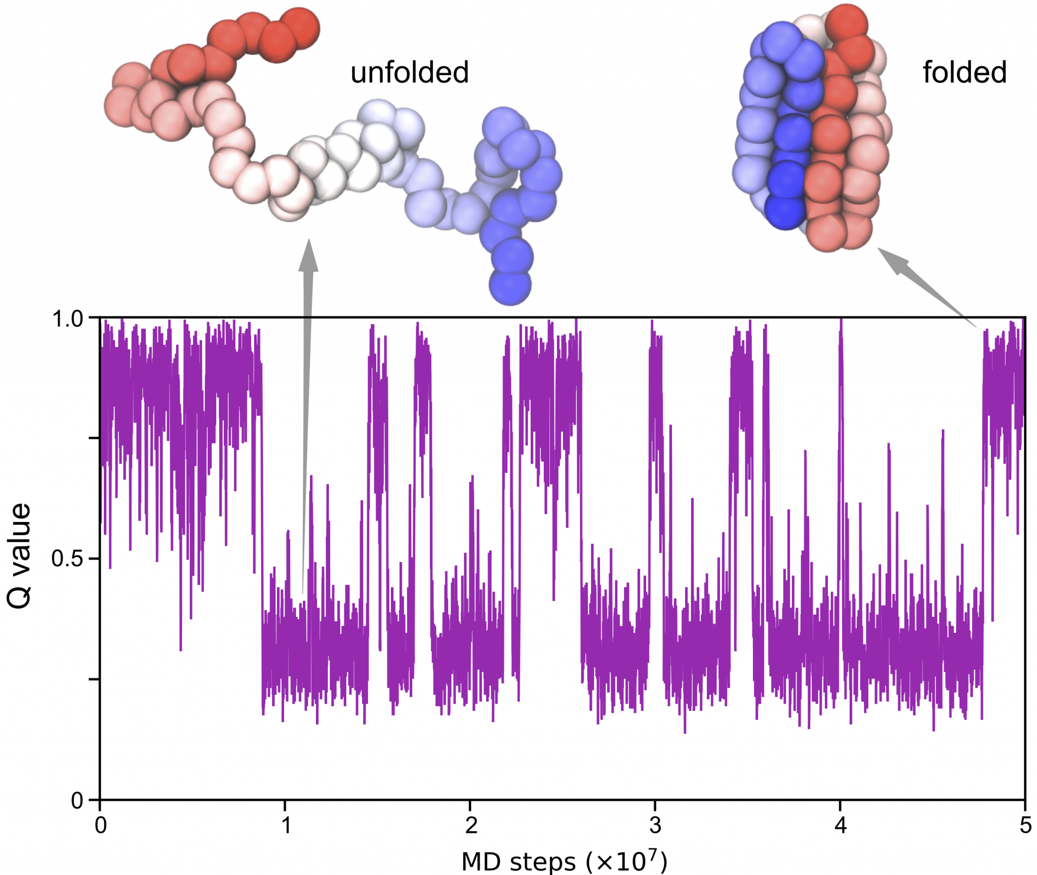
We now make use of the analysis tools packaged in GENESIS to find out more information from CG MD simulations. Here we will try to compute the “Q value” from the trajectory we get in step 2.
Q values are used to estimate the “nativeness” of a conformation and have many different definitions. Here we define the Q value as the fraction of formed native contacts. When the protein is in the folded state, the Q value is high and close to 1.0; whereas when the protein is unfolded, the Q value is low and close to 0.0.
Note that there are two Q-value analysis tools provided by GENESIS, one is
called qval_analysis but used for all-atom Go model; the other is
qval_residcg_analysis and designed for the residue-level CG models. Here we
would like to use the latter one.
$ cd ../03_analysis
$ ls
qval_residcg_analysis.inp
Take a look at this qval_residcg_analysis.inp:
[INPUT]
grotopfile    = ../02_simulation/1PGB_cg.top
grocrdfile    = ../02_simulation/1PGB_cg.gro

[OUTPUT]
qntfile       = pro_md1.qval # nativeness (Q-value) output

[TRAJECTORY]
trjfile1      = ../02_simulation/pro_md1.dcd
md_step1      = 50000000
mdout_period1 = 10000
trj_format    = DCD          # (PDB/DCD)
trj_type      = COOR+BOX     # (COOR/COOR+BOX)

[SELECTION]
group1        = all

[OPTION]
analysis_atom = 1            # group number
lambda        = 1.2          # contact forming distance
The topology (grotopfile) and coordinate (grocrdfile) files are exactly the ones we used to perform the simulation. Native contact information are read from the topology file. For a pair of two CG particles forming a native contact in the native structure, if their distance in a given conformation is within “lambda” times the native value, the contact is considered as formed between them.
$ /home/user/GENESIS/bin/qval_residcg_analysis qval_residcg_analysis.inp
We will get a new file containing the Q values (you may get different values from your simulation):
$ ls
pro_md1.qval

$ head pro_md1.qval
         1  0.98578
         2  0.98578
         3  0.96682
         4  0.83886
         5  0.57346
         6  0.80095
         7  0.83886
         8  0.82464
         9  0.92891
        10  0.92417
Now you can use some data-visualization tools such as gnuplot to
produce a figure of the time series of the Q value:
Written by Cheng Tan@RIKEN Center for Computational Science,
Computational Biophysics Research Team
October, 2021
References
-
Li, W., Wang, W., Takada, S., 2014, Proc. Nation. Acad. Sci., 111, 10550–10555. ↩
-
Clementi, C., Nymeyer, H. & Onuchic, J. N., 2000, Journal of molecular biology 298, 937–953. ↩
-
Tan C., Jung J., Kobayashi C., Ugarte La Torre D., Takada S., and Sugita Y., 2022, PLoS Computational Biology 18(4), e1009578. ↩