GENESIS Tutorial 10.1 (2022)
Acceleration of MD simulations using HMR and a longer time step
Here we show an example how to apply a longer time step than usual by making use of the hydrogen mass repartitioning (HMR) scheme 1, 2, 3 with group temperature/pressure.4 Please note that this option is recommend with accurate temperature/pressure evaluations.4, 5, 6
1. Overview of Hydrogen mass repartitioning (HMR)
In hydrogen mass repartitioning (HMR),1, 2, 3 the mass of hydrogen atoms is
scaled by 2~3 while the mass of the heavy atom bonded to the hydrogen
is reduced such that the total mass is not changed. The figure below is
an example of HMR with a scaling ratio = 3. Here, numbers in each atom
mean atomic
mass.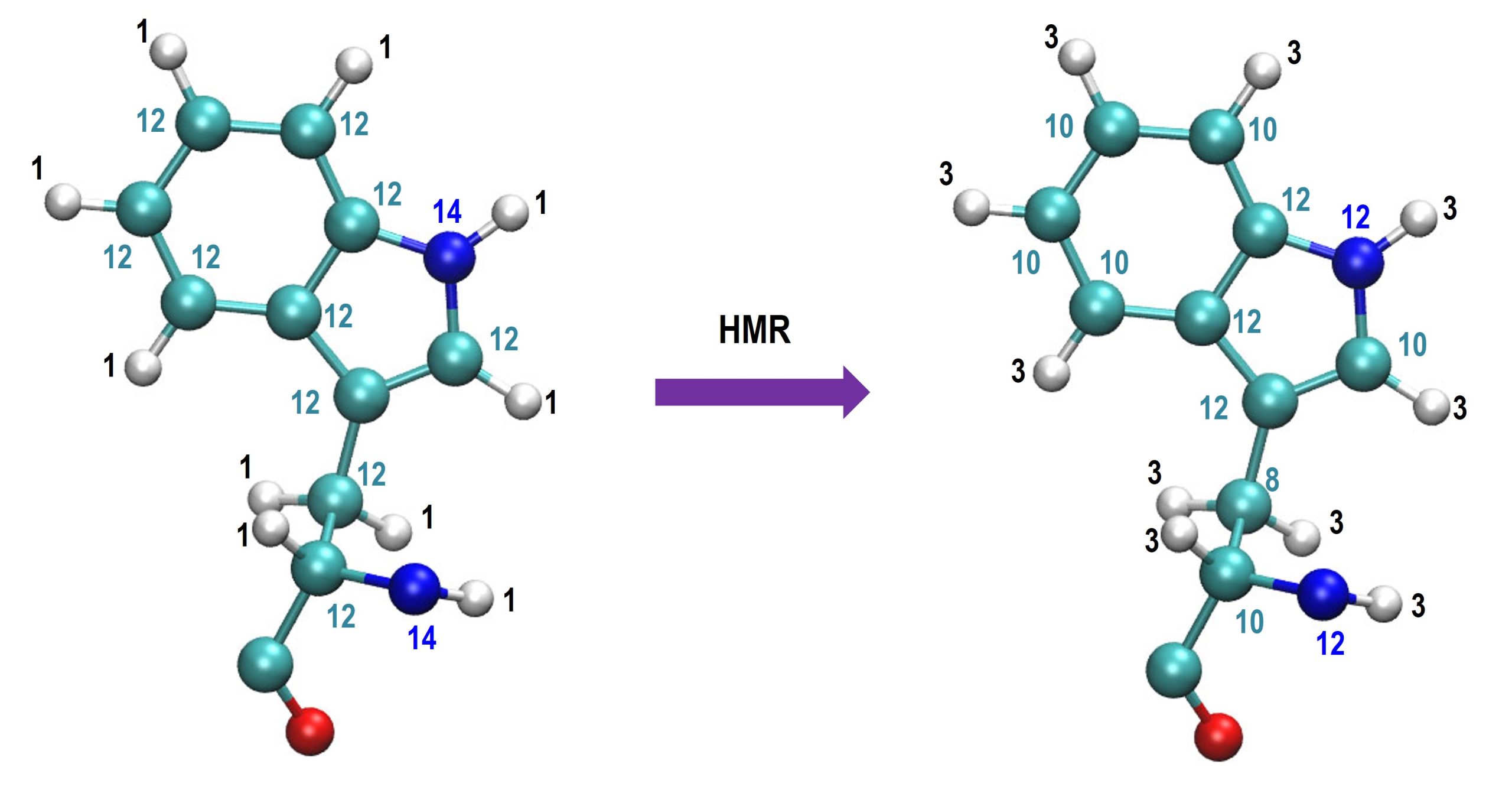
According to our recent investigation, the HMR scaling of hydrogen atoms in five- or six-member rings should be 2 to increase the stability with a large time step, as shown in the figure below:3
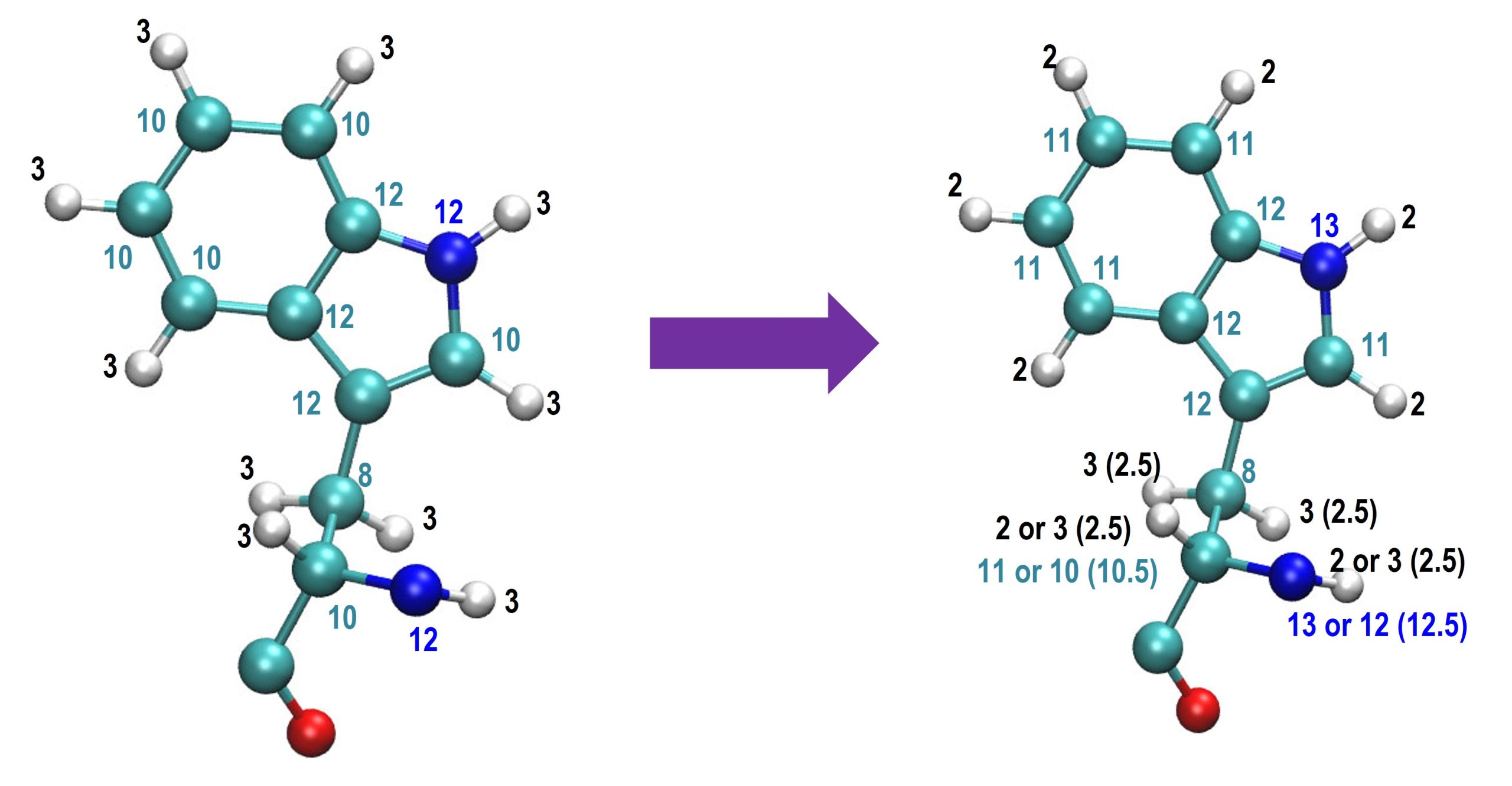
For other hydrogen atoms, we recommend using a HMR scaling ratio of 3 and 2.5 for CHARMM and AMBER force fields, respectively.3 In addition, it is better not to apply HMR to water molecules if you are going to observe dynamic properties from MD. In this tutorial, we will show how to make use of HMR in the simulation of CI2 protein solvated in water molecules. All the input files used in this tutorial can be downloaded in our genesis tutorail github site.
2. Preparations
2.1. Download/Compile GENESIS source code
GENESIS source code can be downloaded from github. After downloading it, you can compile with the following procedure.
$ cd genesis
$ autoreconf
$ ./configure --enable-single
$ make
$ make install
In the case of mixed precision, you can write –-enable-mixed instead
of –-enable-single. For double precision, you don’t need to add
anything. If you are interested in accurate integration with good energy
conservation, we recommend to compile with mixed or double precisions.
Open MPI or Intel MPI libraries can be chosen by writing
# Open MPI
$ ./configure --enable-single FC=mpif90 CC=mpicc
# Intel MPI
$ ./configure --enable-single FC=mpiifort CC=mpiicc
To compile GENESIS on Fugaku or GPU machines, please write as followings:
# Fugaku
$ ./configure --enable-single --host=Fugaku
# GPU
$ ./configure --enable-single –with-cuda={your path of CUDA library}
2.2. Download Tutorial
The input files in this tutorial cover from minimization to production run. After downloading the tutorial file from our github site, you can see five directories and two files.
$ cd cd genesis_tutorial_materials/tutorial-10.1
$ ls
1.min 3.equil_hmr step3_pbcsetup.pdb toppar
2.equil 4.production step3_pbcsetup.psf
3. MD simulation of CI2
To perform the minimization and equilibration runs, you can just follow Level2: STANDARD MD Tutorials. Here, we will present just a brief explanation.
3.1. Minimization
Minimization is the first required step to avoid instability in the structure. The input file is in the [1.min] directory.
$ cd 1.min
$ ls
inp
The content of the Input file is
[INPUT]
parfile = ../toppar/par_all36m_prot.prm
strfile = ../toppar/toppar_all36_prot_c36m_d_aminoacids.str, ../toppar/toppar_water_ions.str
psffile = ../step3_pbcsetup.psf
pdbfile = ../step3_pbcsetup.pdb
reffile = ../step3_pbcsetup.pdb

[OUTPUT]
rstfile = min.rst

[ENERGY]
forcefield       = CHARMM
electrostatic    = PME
switchdist       = 10.0
cutoffdist       = 12.0
pairlistdist     = 13.5
pme_ngrid_x      = 64
pme_ngrid_y      = 64
pme_ngrid_z      = 64
pme_nspline      = 4
water_model      = NONE
vdw_force_switch = YES
contact_check    = YES
nonbond_kernel   = generic

[MINIMIZE]
method          = SD
nsteps          = 1000
rstout_period   = 1000


[BOUNDARY]
type = PBC
box_size_x      = 70
box_size_y      = 70
box_size_z      = 70

[SELECTION]
group1          = (sid:PROA) and backbone
group2          = (sid:PROA) and not backbone and not hydrogen

[RESTRAINTS]
nfunctions      = 2
function1       = POSI
constant1       = 1
select_index1   = 1
function2       = POSI
constant2       = 0.1
select_index2   = 2
In minimization, the contact_check option is often used to avoid
errors when we use an unstable structure in input. In GENESIS v2.0, the
nonbond_kernel is automatically decided from the hardware. However
when contact_check option is used, the generic kernel, which is
identical to the one used in GENESIS 1.7, is assigned.
3.2. Equilibration
In this tutorial, we run equilibration with two steps after the minimization. First, let’s move to the [2.equil] directory.
$ cd ../2.equil
$ ls
inp1 inp2
Here, there are two input files. In inp1, we run the equilibration with
a small time step and with positional restraints. Therefore, there is no
difference between inp1 and minimization input in [INPUT],
[SELECTION], [RESTRAINTS], and [BOUNDARY]. The other sections in
inp1 are written in the following way:
[OUTPUT]
rstfile = equil1.rst
dcdfile = equil1.dcd

[ENERGY]
forcefield       = CHARMM
electrostatic    = PME
switchdist       = 10.0
cutoffdist       = 12.0
pairlistdist     = 13.5
pme_ngrid_x      = 64
pme_ngrid_y      = 64
pme_ngrid_z      = 64
pme_nspline      = 4
vdw_force_switch = YES

[DYNAMICS]
integrator       = VVER
timestep         = 0.001
nsteps           = 100000
crdout_period    = 5000
eneout_period    = 1000
rstout_period    = 100000
nbupdate_period  = 10

[CONSTRAINTS]
rigid_bond       = YES

[ENSEMBLE]
ensemble         = NPT
tpcontrol        = BUSSI
temperature      = 303.15
pressure         = 1.0
In the [ENERGY] section, the contact_check option is not written
based on the assumption that the unstable structure disappeared after
the minimization. rigid_bond in the [CONSTRAINTS] section is defined
to be YES to avoid the vibrational motion of hydrogen atoms. After
running with inp1, you can continue the equilibration with inp2 in which
positional restraints are removed and with 2 fs time step is assigned.
3.3. Equilibration with HMR
If we run an MD simulation with HMR, you can see that the temperature value at the initial step is deviated from the final step of the previous equilibration. To avoid unstable result at initial steps with HMR, it is first recommended to run equilibration with HMR or not to include production results for the first a few ns results. In this tutorial, we will follow the first approach. To make use of HMR, let’s move to [3.equil_hmr] directory.
$ cd ../3.equil_hmr/
$ ls
inp
The input file, inp, is similar to inp2 in [2.equil] directory except
hydrogen_mr   = yes
hmr_ratio     = 3.0
hmr_ratio_xh1 = 2.0
hmr_target    = solute
Here, we scale the mass of hydrogen atoms in the following manner: three
times for for XH2 or XH3 and twice for
XH1 (where X and H represent any heavy and hydrogen atoms, repsectively).
In addition, HMR is not applied water molecules. To make use of the HMR
option, first please write hydrogen_mr = yes. If not, HMR is not
applied even if you write HMR related keys in the control input file.
The HMR scaling ratio is controlled by hmr_ratio. It scales up the
mass of hydrogen atoms while the mass of the bonded heavy atom is
reduced to conserve the total mass. hmr_ratio_xh1 scales the mass of
hydrogen atoms in XH1.
Please note that HMR input in GENESIS is distinguished from NAMD or AMBER program. In NAMD and AMBER, the scaled hydrogen mass should be written directly in the psf and prmtop files, respectively. For example, the psf files with and without HMR scaling are written as following:
#psf without HMR
 32413 !NATOM
1 PROA 20 MET N   NH3 -0.300000 14.0070 0 0.00000 -0.301140E-02
2 PROA 20 MET HT1 HC   0.330000 1.00800 0 0.00000 -0.301140E-02
3 PROA 20 MET HT2 HC   0.330000 1.00800 0 0.00000 -0.301140E-02
4 PROA 20 MET HT3 HC   0.330000 1.00800 0 0.00000 -0.301140E-02
5 PROA 20 MET CA  CT1  0.210000 12.0110 0 0.00000 -0.301140E-02
6 PROA 20 MET HA  HB1  0.100000 1.00800 0 0.00000 -0.301140E-02
. . .

#psf with HMR
 32413 !NATOM
1 PROA 20 MET N   NH3 -0.300000 7.95900 0 0.00000 -0.301140E-02
2 PROA 20 MET HT1 HC   0.330000 3.02400 0 0.00000 -0.301140E-02
3 PROA 20 MET HT2 HC   0.330000 3.02400 0 0.00000 -0.301140E-02
4 PROA 20 MET HT3 HC   0.330000 3.02400 0 0.00000 -0.301140E-02
5 PROA 20 MET CA  CT1  0.210000 9.99500 0 0.00000 -0.301140E-02
6 PROA 20 MET HA  HB1  0.100000 3.02400 0 0.00000 -0.301140E-02
 . . .
In this example, the masses of hydrogen atoms with HMR become three times larger (1.008 to 3.024) in the psf file, while the masses of boned heavy atoms are reduced accordingly. Therefore, psf files should be regenerated to perform MD with HMR. Similarly, masses in an AMBER parameter file are changed to apply HMR:
# parameter without HMR
%FLAG MASS
%FORMAT(5E16.8)
1.40070000E+01 1.00800000E+00 1.00800000E+00 1.00800000E+00 1.20110000E+01
1.00800000E+00 1.20110000E+01 1.00800000E+00 1.00800000E+00 1.20110000E+01
 . . .

# parameter with HMR
%FLAG MASS
%FORMAT(5E16.8)
7.95900000E+00 3.02400000E+00 3.02400000E+00 3.02400000E+00 9.99500000E+00
3.02400000E+00 7.97900000E+00 3.02400000E+00 3.02400000E+00 7.97900000E+00
Unlike them, we do not have to change psf or parameter files. Instead we just write the HMR option, and program automatically performs simulations with scaled hydrogen masses.
3.4. Production run with HMR
After you equilibrate with HMR, you can run MD simulations with a large time step. Let’s move to the directory of production runs ([4.production]).
$ cd ../4.production/
$ ls
inp1 inp2 inp2_nohmr
In inp1, we perform production run with multiple time step with 3.5 fs for the short time step and 7.0 fs for the long time step. In inp2 and inp2_nohmr, we perform production run with 5 fs time step with and without HMR, respectively. Main differences in the control inputs are shown as following:
inp1:

[DYNAMICS]
integrator        = VRES
timestep          = 0.0035
nsteps            = 120000
crdout_period     = 3000
eneout_period     = 60
rstout_period     = 120000
nbupdate_period   = 6
hydrogen_mr       = yes
hmr_ratio         = 3.0
hmr_ratio_xh1     = 2.0
hmr_target        = solute
thermostat_period = 6
barostat_period   = 6

inp2:

[DYNAMICS]
integrator        = VVER
timestep          = 0.005
nsteps            = 100000
crdout_period     = 2000
eneout_period     = 50
rstout_period     = 100000
nbupdate_period   = 4
hydrogen_mr       = yes
hmr_ratio         = 3.0
hmr_ratio_xh1     = 2.0
hmr_target        = solute
thermostat_period = 4
barostat_period   = 4

inp2_nohmr:

[DYNAMICS]
integrator        = VVER
timestep          = 0.005
nsteps            = 100000
crdout_period     = 2000
eneout_period     = 50
rstout_period     = 100000
nbupdate_period   = 4
thermostat_period = 4
barostat_period   = 4
Here, we note that crdout_period (period of trajectory writing output), rstout_period (period of restart file writing output),
nbupdate_period (period of pairlist updating), thermostat_period
(period of thermostat), and barostat_period (period of barostat)
should be adjusted such that the total update interval should not be
changed.
The effect of HMR can be understood by running inp2 and inp2_nohmr. We could run inp2 without any problem. On the other hand, running inp2_nohmr has an error message in constraints:
Compute_Shake> SHAKE algorithm failed to converge: indexes 775 776 777
In other words, the MD simulation with a large time step is not stable without HMR assignment.
With optimal temperature estimation, atomic temperature and pressure
evaluations require iterations when rigid_bod=yes is used in
[CONSTRAINTS]. To avoid the iteration, we recommend using group
temperature and pressure evaluations by writing group_tp=yes in the
[ENSEMBLE] section.
Written by Jaewoon Jung@RIKEN R-CCS.
March, 2022
Updated by Jaewoon Jung@RIKEN R-CCS.
June, 23, 2022
Updated by Jaewoon Jung@RIKEN R-CCS.
June, 10, 2025
4. References
-
K. A. Feenstra, B. Hess, and H. J. C. Berendsen, 1999, J. Comput. Chem., 20, 786–798 ↩ ↩2
-
C. W. Hopkins, S. Le Grand, R. C. Walker, and A. E. Roitberg, 2015, J. Chem. Theory Comput., 11, 1864–1874 ↩ ↩2
-
J. Jung, K. Kasahara, C. Kobayashi, H. Oshima, T. Mori, and Y.Sugita, 2021, J. Chem. Theory Comput., 17, 5312–5321 ↩ ↩2 ↩3 ↩4
-
J. Jung and Y. Sugita, 2020, J. Chem. Phys., 153, 234115 ↩ ↩2
-
J. Jung, C. Kobayashi and Y. Sugita, 2019, J. Chem. Theory Copmput. 15, 84–94 ↩
-
J. Jung, C. Kobayashi and Y. Sugita, 2018, J. Chem. Phys., 148, 164109 ↩