GENESIS Input Example: Radial distribution function (rdf_analysis)
rdf_analysis calculates conventional radial distribution function (RDF) and
proximal distribution function (PDF) of the target solvent atoms. In both
functions, the available volumes \(V(r)\) (see below), and the coordination
number of the solvent atoms in the available volume \(N(r)\) are calculated.
The number density of the solvent \(\rho(r)\) is obtained as \(\rho(r) =
N(r)/V(r)\). The profile is calculated until buffer (Å), and output until
range (Å) with the bin size (\(\Delta r\)) = binsize (Å).
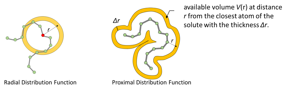
The option rmode=proximal calculate PDF. PDF gives number density of selected
solvent atoms as a function of the distance from the closest atom of the solute.
Resolution (=size of a cell) is determined by num_cell_x,y,z. When the
trajectory is generated by NPT condition, the resolution fluctuates in
conjunction with the fluctuation of box size. Therefore, rdf_analysis should not
apply on the trajectory in which the box size is not converged enough. In order
to obtain the normalized profile, atomic number density in each bin should be
divided by bulk density. The option bulk_region means that the last
bulk_region (%) of the un-normalized number density profile is averaged and
the averaged density is adopted as bulk density. In stead of this automatic
normalization, the option bulk_value can specify the bulk density manually.
The option recenter may improve the load balance between MPI process, but
please make sure that the coordinate of the target solute molecule is not
separated by the periodic boundary condition.
(EX1) Proximal distribution function (PDF) of water oxygen around a BPTI
This input calculates the PDF of water oxygen atoms around a protein BPTI
(group1) in water box with PBC. In this example, resolution (= size of a cell)
is around 0.5 Å3. The profile is calculated, and output until 10 Å
from the closest (selected) BPTI atoms. The histogram is taken with the bin size
(binsize) = 0.5 Å. The bulk density is determined using the last 15%
(specified by the option bulk_region) of the un-normalized density profile.
[INPUT]
psffile = ionize.psf
reffile = ionize.pdb
pdbfile = ionize.pdb

[OUTPUT]
txtfile = bpti_proximal.out

[TRAJECTORY]
trjfile1      = run.dcd
md_step1      = 500000
mdout_period1 = 500
ana_period1   = 5000
repeat1       = 1
trj_format    = DCD
trj_type      = COOR+BOX

[BOUNDARY]
type = PBC
box_size_x     = 68.25815
box_size_y     = 80.24045
box_size_z     = 66.58892
domain_x       = 2
domain_y       = 2
domain_z       = 2
num_cells_x    = 136
num_cells_y    = 160
num_cells_z    = 132

[ENSEMBLE]
ensemble = NPT

[SELECTION]
group1 = ai:1-892
group2 = rnam:TIP3 and an:OH2

[SPANA_OPTION]
buffer = 10
wrap     = yes
box_size = TRAJECTORY

[RDF_OPTION]
rmode       = proximal
solute      = 1
solvent     = 2
binsize     = 0.25
range       = 10
bulk_region = 15.0
recenter    = 1
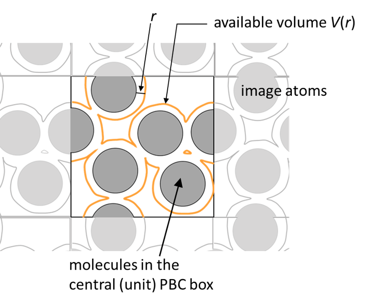
(EX2) proximal distribution function of water oxygen around multiple villins under the crowding condition
This example calculates the PDF for multiple villins under the crowding
condition. All villin atoms specified by group1 in the [SELECTION] are
uniformly recognized as the component of a solute. When boundary type is PBC,
rdf_analysis takes account the image atoms around the unit box.
[INPUT]
psffile = villin_crowding.psf
reffile = villin_crowding.pdb
pdbfile = villin_crowding.pdb

[OUTPUT]
txtfile = villin_proximal.out

[TRAJECTORY]
trjfile1      = prod.dcd
md_step1      = 10000
mdout_period1 = 500
ana_period1   = 500
repeat1       = 1
trj_format    = DCD
trj_type      = COOR+BOX

[BOUNDARY]
type = PBC
box_size_x   = 142
box_size_y   = 142
box_size_z   = 142
domain_x     = 2
domain_y     = 2
domain_z     = 2
num_cells_x  = 142
num_cells_y  = 142
num_cells_z  = 142

[ENSEMBLE]
ensemble = NVT

[SELECTION]
group1 = ai:1-13112
group2 = rnam:TIP3 and an:OH2

[SPANA_OPTION]
buffer   = 10
wrap     = yes
box_size = TRAJECTORY

[RDF_OPTION]
rmode    = proximal
solute   = 1
solvent  = 2
binsize  = 0.5
range    = 8
(EX3) Radial distribution function between oxygen atoms in TIP4P water box
The option rmode=radial calculate RDF. The number densities of the solvent
atoms around each solute atom are calculated, and the ensemble average over
those values is output. In this example, all oxygen atoms in the system are
selected, and all pair for those oxygen atoms are analyzed. If the number of the
solvent molecule is too large, it is better to thin out the solute atoms (e.g.,
by limiting the atom index like, group1 = ai:1-10000 and an:OH2)
[INPUT]
psffile = solvate.psf
reffile = solvate.pdb
pdbfile = solvate.pdb

[OUTPUT]
txtfile = tip4p_radial.out

[TRAJECTORY]
trjfile1      = genesis_tip4p_nvt.dcd
md_step1      = 500000
mdout_period1 = 500
ana_period1   = 500
repeat1       = 1
trj_format    = DCD
trj_type      = COOR+BOX
trj_natom     = 0

[BOUNDARY]
type = PBC
box_size_x     = 57
box_size_y     = 57
box_size_z     = 57
domain_x       = 2
domain_y       = 2
domain_z       = 2
num_cells_x    = 20
num_cells_y    = 20
num_cells_z    = 20

[ENSEMBLE]
ensemble = NVT

[SELECTION]
group1   = an:OH2
group2   = an:OH2

[SPANA_OPTION]
buffer   = 10
wrap     = yes
box_size = TRAJECTORY

[RDF_OPTION]
rmode       = radial
solute      = 1
solvent     = 2
binsize     = 0.5
range       = 10
bulk_region = 15